Python
Status: This page is work in progress...
Last changed: Saturday 2015-01-10 18:32 UTC
Abstract:
Python is a high-level programming language first released by Guido van Rossum in 1991. Python is designed around a philosophy which emphasizes readability and the importance of programmer effort over computer effort. Python core syntax and semantics are minimalist, while the standard library is large and comprehensive. Python is a multi-paradigm programming language (primarily functional, object oriented and imperative) which has a fully dynamic type system and uses automatic memory management -- it is thus similar to Perl, Ruby, Scheme, and Tcl. The language has an open, community-based development model managed by the non-profit Python Software Foundation. While various parts of the language have formal specifications and standards, the language as a whole is not formally specified. The de facto standard for the language is the so-called CPython implementation. Some of the largest projects that use Python are the Zope application server, the Mnet distributed file store, YouTube, and the original BitTorrent client. Large organizations that make use of Python include Google and NASA. Air Canada's reservation management system is written in Python. Python has also seen extensive use in the information security industry -- it is commonly used in exploit development. Also, Python has been successfully embedded in a number of software products as a scripting language. For many OSs (Operating Systems), Python is a standard component -- it ships with most Linux distributions, with FreeBSD, NetBSD, and OpenBSD, and with Mac OS X. From a developers point of view, Python has a large standard library, commonly cited as one of Python's greatest strengths, providing tools suited to many disparate tasks. This comes from a so-called "batteries included" philosophy for Python modules. The modules of the standard library can be augmented with custom modules written in either C or Python. Recently, Boost C++ Libraries includes a library, python, to enable interoperability between C++ and Python. Because of the wide variety of tools provided by the standard library combined with the ability to use a lower-level language such as C and C++, which is already capable of interfacing between other libraries, Python can be a powerful glue language between languages and tools. This page is going to cover various aspects of Python and programming in Python as seen from a developers point of view. Last but not least, note that this page is about Python 3 where applicable and only refers to Python 2 where still necessary at the point of writing.
|
Table of Contents
|
Python, it just fits your brain...
— unknown
Introduction
This sections features as a general get to know Python section in that
it touches on the most profound theoretical and practical subjects.
First thing to remember about Python is
... in Python everything is an object!
-
Strings are objects. Lists are objects. Functions are objects. Classes
are objects. Class instances are objects. Properties are objects.
Modules are objects. Files are objects. Network connections are
objects. Descriptors are objects.... this list goes on and on...
Second most important thing with regards to Python is that
Iterators are everywhere, underlying everything, always just
out of sight.
Both, iterators and objects are explained in detail further down...
Main Usage Areas
So what is it that most people use Python for? Well, there are two
main usage areas:
- Web Applications and
- System Administration and Automation
There are many others too like for example scientific computing or
robotics but those are areas which have a considerably smaller
userbase than the two major areas mentioned above.
Why Python?
Python where we can, C++ where we must... As with many things in
live, simplicity is key. Even more so if by gaining simplicity we do
not have to cut back on features but maybe even gain on both ends.
Wow! Guess what, that thing exists and it goes by the name Python:
Python where we can, C++ where we must — they used (a subset of) C++
for the parts of the software stack where very low latency and/or
tight control of memory were crucial, and Python, allowing more rapid
delivery and maintenance of programs, for other parts.
If you are asking yourself Who are they? in this context, the answer
is: The founders of Google. So, why might someone make the decision
for this technology stack? Easy:
If I can write 10 lines of code in language X to accomplish what took you
100 lines of code in language Y, then my language is more powerful.
or in other words
>>> if succinctness == power:
...     print("You are using Python.")
...
...
You are using Python.
>>>
Again you see, simplicity is good, simplicity scales, simplicity
shortens product cycles, simplicity helps reduce time to market and
last but not least, simplicity is more fun — heck, I would rather
spend a few hours and write some useful piece of software rather than
debugging some arcane memory bug in an even more arcane programming
language. Been there, done that...
Everything should be made as simple as possible, but not simpler.
— Albert Einstein
With the following subsections we are going to look at why/what that
often mentioned simplicity might be. I know you want facts, and
rightfully so!
Philosophy
It is important for anyone involved with Python to at least understand
a few basic/core ideas about the language itself:
- Python is FLOSS (Free/Libre Open Source Software) i.e. it is
developed by many rather than one individual or company. There are
no license fees that need to be paid for using it, there is no
risk of a vendor lock-in i.e. developing in Python gives
investment security.

- Python is a high-level programming language i.e. it is a
programming language with strong abstraction from the details of
the computer. Any high-level programming languages generally hides
the details of CPU operations such as memory access models and
management of scope. In comparison to low-level programming
languages, Python has more natural human language elements and its
code is portable across many hardware platforms and operating
systems.
- From a programming paradigm point of view, Python is a
multi-paradigm programming language. A multi-paradigm programming
language is a programming language that supports more than one
programming paradigm e.g. object oriented, functional, aspect
oriented, etc. The basic idea of a multiparadigm programming
language is to provide a framework in which programmers can work
in a variety of styles, freely intermixing constructs from
different paradigms. The design goal of such languages is to allow
programmers to use the best tool for a job, admitting that no one
paradigm solves all problems in the easiest or most efficient way.
- Python is known for its well thought out and easily readable
syntax (e.g. indentation) which in turn boosts productivity and
also makes it a great language for beginners.
- Python is a dynamic language with an dynamic type system. However,
despite having a dynamic type system, Python is strongly typed.
- The automatic memory management of Python is based on its dynamic
type system and a combination of reference counting and
garbage collection.
- Python is fully Unicode aware. There is also excellent support for
internationalization and localization.
- From the very beginning, the overall design concept of Python has
been: Keep the core language to a minimum and provide a large
standard library and means to easily extend the core with own code
and/or third party code.
- Python's philosophy rejects the thinking of there is more than one
way to do it approach to language design in favor of there should
be one (and preferably only one) obvious way to do it.
- As we know, premature optimization is the root of all evil.
Therefore, when speed is a problem, Python programmers tend to
try to optimize bottlenecks by algorithm improvements or data
structure changes, using a JIT (just-in-time compilation)
compiler such as Psyco, rewriting the time-critical functions in
closer to the metal languages such as C, or by translating Python
code to C code using tools like Cython.
Random Stuff
There are quite a few random things eventually interesting...
History of Python
1991 - Dutch programmer Guido van Rossum travels to Argentina
for a mysterious operation. He returns with a large cranial
scar, invents Python, is declared Dictator for Life by legions
of followers, and announces to the world that "There Is Only One
Way to Do It." Poland becomes nervous.
Those who are looking for a serious answer, go use some search engine
;-]
Zen of Python
>>> import this
The Zen of Python, by Tim Peters

Beautiful is better than ugly.
Explicit is better than implicit.
Simple is better than complex.
Complex is better than complicated.
Flat is better than nested.
Sparse is better than dense.
Readability counts.
Special cases aren't special enough to break the rules.
Although practicality beats purity.
Errors should never pass silently.
Unless explicitly silenced.
In the face of ambiguity, refuse the temptation to guess.
There should be one -- and preferably only one -- obvious way to do it.
Although that way may not be obvious at first unless you're Dutch.
Now is better than never.
Although never is often better than *right* now.
If the implementation is hard to explain, it's a bad idea.
If the implementation is easy to explain, it may be a good idea.
Namespaces are one honking great idea -- let's do more of those!
>>>
Everything written in Python should adhere to those principles. Things
like frameworks which are written in Python might have
additional principles/conventions on top of the ones outlined above.
In addition, there are coding styles which we should adhere.
Cheat Sheet or RefCard
Yes, the Internet has plenty of resources on the matter. Here is one
of them.
Quickstart
This subsection is a summary of the semantics and the syntax found in
Python. It can be read and followed along on the command line in less
than an hour.
It is intended as a glance into Python for those who have not had
contact with Python yet, or, for those who want a quick refresh of the
cornerstones that makeup for most of Python's look and feel. Also,
without further notice, note that this page is about Python 3 where
applicable and only refers to Python 2 where still necessary at the
point of writing.
One of the things I like most about Python is that it is not as wordy
as Java/C++ and not as cryptic as Perl but just a programming language
with an pragmatic approach to software development — something I
would also love to see for JavaScript, which somehow has become my
second most used programming language right after Python and before
Java/C++. Enough said, let us now go and ride the snake a little...
Preparations
It is strongly recommended to follow along using Python's built-in
interactive shell. Personally I prefer to use bpython but then the
standard built-in shell is just fine.
One needs to install Python if not installed already e.g. using APT
(Advanced Packaging Tool) by issuing aptitude install python or
install it manually. After installing one should be able to find the
interpreter and start the interactive shell:
sa@wks:~$ which python
/usr/bin/python
sa@wks:~$ python3
Python 3.2 (r32:88445, Feb 20 2011, 19:50:20)
[GCC 4.4.5] on linux2
Type "help", "copyright", "credits" or "license" for more information.
>>>
As of now (November 2011) /usr/bin/python still links to Python 2 as
standard Python instead of Python 3 in which case we simply have to
specify python3 as I did above. Also, Python 3 needs to be installed
of course: aptitude install python3 — it is no problem to have both
Python versions installed at the same time. Before we actually start,
let us make sure we run Python 3. I always use bpython and just issue
python because I have some magic that fires up Python 3 and does some
initialization... anyhow, the only thing one needs to know is that
aptitude install python3 installs Python 3python3 starts the interactive shell on Python 3sysconfig.get_python_version() allows us to check which Python
version we are running, just to be sure
Ok, grab your helmets, fasten seat belts... turn ignition...
Basics
Assignment, values, names and the print() function:
>>> foo = 3                     # bind (through assignment) name foo to value 3
>>> print(foo)                  # use print function on object foo
3
>>> bar = "hello world"         # a string is a value too
>>> print(bar)
hello world
>>> fiz = foo                   # bind name fiz to the same value foo is bound to already
>>> print(fiz)
3
>>>
Expressions and statements:
>>> 3 + 2                       # an expression is something
5
>>> print(3 + 2)                # a statement does something
5
>>> len(bar)                    # another statement
11
>>>
Code blocks are set apart using whitespace rather than braces.
Conditionals, clauses and loops work as one would expect:
>>> for character in "abc":
...     print(character)                        # 4 spaces per indentation level
...
...
a
b
c
>>> for character in "abc":
...     print(character)
...     if character in "a":
...         print("found character 'a'")        # 8 spaces on level 2
...
...
...
a
found character 'a'
b
c
>>> if 4 == 2 + 2:
...     print("boolean context evaluated to true")
...
... else:
...     print("boolean context evaluated to false")
...
...
boolean context evaluated to true
>>>
Mostly the semantics of while loops can be done more efficiently using
for loops and operators such as in. This is especially true in case we
need a counter in order iterate through a sequence — absent the fact
that when in need of a counter, the experienced Pythoneer would
probably turn to a closures anyway.
Following the link about counters also shows us the use of the range()
function, maybe one of the most used functions next to print() and a
few others. Also, by now it should be clear that lines beginning with
# or everything following a # is a comment, thus ignored by Python.
Data Structures
With only a few built-in Python data structures we can probably cover
80% of use cases. To get to 100% we can then use third party add-ons
(so-called packages and/or modules) written by others or simply build
our custom data structures and maybe also some custom algorithms which
we purposely designed to go with our custom data structures.
Relations amongst Data Structures
We have already seen some data structures — numbers and strings.
Numbers are so-called literals whereas strings are sequences.
Sequences itself are a subset of containers, which in turn is not just
the superset to sequences but also to mappings and sets.
What all data structures have in common is that each of them is either
itself an object or some sort of grouping thereof. Another thing that
is true for any data structure is that it is either mutable (can be
modified in place) or immutable (cannot be modified in place) — place
being location(s) in memory.
Below is a sketch picturing what we just said about how data
structures in Python relate (formatting does not carry any information
but was chosen to make things fit):
                                    o     b     j     e     c     t
                                    /                             \
                                   /                               \
                               literals                        c    o    n    t    a    i    n    e    r    s
                                /   \                          /                        |                   \
                               /     \                        /                         |                    \
                       immutable    mutable        s e q u e n c e s              m a p p i n g s           s e t s
                        /     \                    /               \                /           \           /     \
                       /       \                  /                 \              /             \         /       \
          n u m b e r s        etc.       immutable               mutable       mutable     immutable  immutable   mutable
          /     |     \                  /   |    \               /  |           /                        /          \
         /      |      \                /    |     \             /   |          /                        /            \
    integral  complex  real/float  strings  tuples  etc.     lists  etc.    dictionaries               frozenset      set
     /   \             /       \                                              /        \
    /     \           /         \                                            /          \
 integer  boolean  decimal    binary                                  OrderedDict       etc.
The sketch, even if it is not complete but only shows the root and a
few branches, is a good enough approximation and should help with
understanding how data structures in Python relate — they are
basically arranged in a tree structure, based on semantics they carry.
Numbers, Lists, Tuples, Dictionaries
Numbers/Integers
>>> 2
2
>>> type(2)                             # check for class/type
<class 'int'>                           # yes, 2 is indeed an integer
Numbers/Floats:
>>> 1.1 + 2.2
3.3000000000000003
>>> type(1.1)
<class 'float'>
Lists
>>> foo = [2, 4, "hello world"]         # create a lists with three items
>>> type(foo)
<class 'list'>
>>> foo[0]                              # get item at index position 0
2
>>> foo[2]
'hello world'
>>> foo[2] = "hello big world"          # assign to index position 2
>>> foo
[2, 4, 'hello big world']               # assignment worked because lists are mutable
>>> foo[1:]                             # get a slice
[4, 'hello big world']
>>> foo[:-1]                            # slice but with negative upper boundary
[2, 4]
>>> foo[-1:]                            # negative lower boundary
['hello big world']
Tuples
>>> bar = (2, 4, "hello world")
>>> type(bar)
<class 'tuple'>
>>> bar[0]
2
>>> bar[2]
'hello world'
>>> bar[2] = "hello big world"
Traceback (most recent call last):      # because tuples are immutable
  File "<input>", line 1, in <module>
TypeError: 'tuple' object does not support item assignment
>>> bar
(2, 4, 'hello world')
>>> bar[1:]                             # same as for lists
(4, 'hello world')
Dictionaries
- we are going to create a dictionary with three key/value pairs also
known as items
- keys need to be immutable; values can be both, immutable and mutable
- dictionaries are unordered i.e. the order of items is not
guaranteed (see how
foobar changes position from last to first)
>>> fiz = {'foo': 3, 'baz': "hello world", 'foobar': bar}               # using bar from above
>>> type(fiz)
<class 'dict'>
>>> fiz
{'foobar': (2, 4, 'hello world'), 'baz': 'hello world', 'foo': 3}
>>> fiz['foo']
3
>>> fiz['foobar']
(2, 4, 'hello world')
>>> fiz['baz'] = "hello big world"
>>> fiz['baz']
'hello big world'
>>> fiz
{'foobar': (2, 4, 'hello world'), 'baz': 'hello big world', 'foo': 3}
>>> fiz['foobar'][1]                                                    # nested
4
>>>
Built-in Goodies
So far we have only scratched the subject of built-in data structures
in Python. We already know that each data structure is in fact an
object. This object holds some sort of data e.g. a list has items.
It is not far of to think that it would be nice if those objects also
had ways to operate on the data they store e.g. reverse the items of
a list etc. Guess what, that is exactly the case — every data
structure comes with ready-made functionality to operate on the data
it stores! Let us just have a quick look at a few:
>>> foo
[2, 4, 'hello big world']
>>> foo.reverse()                       # works because lists are mutable
>>> foo
['hello big world', 4, 2]
>>> bar.count(4)                        # number occurrences of value 4 in tuple bar
1
>>> bar.index(2)                        # index position of value 2
0
>>> fiz.items()
dict_items([('foobar', (2, 4, 'hello world')), ('foo', 3), ('baz', 'hello big world')])
>>> fiz.keys()
dict_keys(['foobar', 'foo', 'baz'])
>>> fiz.values()
dict_values([(2, 4, 'hello world'), 3, 'hello big world'])
>>>
By the way, those built-in goodies are actually method objects linked
to from each data structure instance but let us not get ahead of
ourselves for now...
Functions
The next step is to combine all we have seen so far and group behavior
(code) in order to more efficiently manage state (data). Functions are
basically just code blocks (set apart by indentation) which we can
refer to by name and which body contains statements and expression
which semantically belong together.
However, grouping is just one thing that is nice about using
functions. Being able to refer to code blocks by name is nice too.
However, where the real benefit comes into play is when we start
reusing those code blocks in order to avoid code duplication.
>>> def amplify(foo):                   # function signature; foo is its only parameter
...     print(foo * 3)                  # function body
...
...
>>> amplify('hi')                       # works for strings
hihihi
>>> amplify(2)                          # and numbers...
6
>>> type(amplify)
<class 'function'>
>>> bar = amplify                       # now bar and amplify, both are bound to
>>> type(bar)
<class 'function'>
>>> bar is amplify                      # the same function object
True
>>> bar
<function amplify at 0x24f3490>         # 0x24f3490 address of function object in memory
>>> amplify
<function amplify at 0x24f3490>
>>> bar(2)
6
>>>
The most important thing to understand about functions is that they
are objects too, just like strings etc. What that means is that we can
assign them to arbitrary names — like we just did when we bound the
name bar (through assignment) to the function object located at memory
address 0x24f3490. Again, that is two (or more) names bound to one
object!
It is also important to understand that functions can take arguments,
something quite important when we want to reuse code where the
processing (read code/logic) stays the same but of course input data
varies (e.g. can be hi or 2 or whatever, as shown above).
At this point there is no need to concern ourselves with the concepts
of scope and namespaces, as we will see more on them later. The last
thing which is certainly necessary to know with regards to functions
is that they always return something.
Custom Data Structures
Next to many built-in data structures we can create our custom ones —
the terms class/type, superclass/supertype, subclass/subtype, instance
and OOP (Object-Oriented Programming), all hint that we are dealing
with custom data structures. I advice people to maybe go visit each of
those links, maybe read the first one or two paragraphs and then come
back for a light introduction into custom data structures in Python:
 1  >>> class Foo:                                                             # creating a class/type
 2 ...     pass
 3 ...
 4 ...
 5  >>> type(Foo)
 6  <class 'type'>
 7  >>> class Bar(Foo):                                                        # subclassing
 8 ...     def __init__(self, firstname=None, surname=None):                   # a (special) method
 9 ...         self.firstname = firstname or None
10 ...         self.surname = surname or None
11 ...
12 ...     def print_name(self):                                               # another method
13 ...         print("I am {} {}.".format(self.firstname, self.surname))
14 ...
15 ...
16 ...
17  >>> type(Bar)
18  <class 'type'>
19  >>> Bar.__bases__
20  (<class '__main__.Foo'>,)
21  >>> aperson = Bar(firstname="Niki", surname="Miller")                       # instantiating
22  >>> isinstance(aperson, Bar)
23  True
24  >>> isinstance(aperson, Foo)
25  True
26  >>> aperson.print_name()                                                    # method call
27  I am Niki Miller.
28  >>>
In only 28 lines we have shown about 90% there is to know about custom
data structures in Python. In line 1, we use the class keyword to
create a new class/type — let me thrown in a referrer to
naming conventions now for the first time. We then use pass in the
class body because, actually, we do not want to use Foo for anything
other than subclassing Bar from it in line 7.
With Bar we actually implement a few things — why not create a custom
data structure used to store basic information related to a person,
such as his/her name. Yes, let us do that!
Since a class/type is basically a blueprint used to create instances
from, every instance (individual person in our case) will have a
different name of course. We want to store a persons name
automatically right after creating the instance i.e. when it gets
initialized — that is what the __init__() special method does,
initialising a fresh-out-of-the-oven instance.
We can put whatever we want into the body of __init__(), such as for
example grabbing the information about a persons name provided to us
when an instance is created. We then store the name on the instance
(lines 9 and 10).
That is what self is used for... referencing the instance in question
i.e. either accessing already stored information (line 13) or storing
information (lines 9 and 10) on an instance of some class/type.
Also, note the use of or which in our current case means that only if
we provide e.g. firstname when instantiating (line 21), is it stored
on the instance (self.firstname). If we do not provide it, None is
automatically stored (or whatever follows or in lines 9 and 10; not to
be confused with None from the function signature in line 8, that is
the default parameter value, which just happens to be None as well).
We already know the built-in type() function from above, we use it to
find out to which class/type a certain name is bound to. In our case
it is type type, twice, lines 6 and 18. Let us not worry about type
for now. What is more interesting and of more practical use is a
closer look at the concept of inheritance since we subclassed Bar from
Foo — no special reason really, just to showcase how subclassing is
done i.e. we could have put lines 8 to 13 instead of lines 2 and be
fine without ever creating Bar.
Line 22 and 23 show how we can check whether or not aperson really is
an instance of Bar. And guess what, since Bar is a subclass of Foo (or
looked at it the other way around, Foo a superclass/supertype to Bar)
aperson is of course also a instance of Foo (lines 24 and 25).
print_name is a method (the other name for functions when defined
inside a class/type) which means that aside from the fact that it has
the implicit self argument, it really is a function under the hood,
the stuff we already looked at above. Line 26 shows how we call a
method which now lives on (or actually is referenced from) the aperson
instance. () is the call operator.
Last but not least, a word on inheritance... The nifty thing from
line 19 and 20 is using a so-called class/type attribute to see if Bar
in fact has a superclass/supertype other than the built-in Python one
i.e. if it is the topmost not Python built-in class/type within the
inheritance chain or not. Turns out it is not because it is subclassed
from Foo.
Standard Library
It is a must for any Pythoneer to know about the
Python standard library, what it contains, as well as
how and when to use it. It has lots of useful code, highly optimized,
for many problems seen by most people over and over again for all
kinds of problem domains across many industries. Using bits and pieces
form the standard library always starts with importing code which can
then be used right away. Let us look at some examples:
>>> import math
>>> math.pi
3.141592653589793
>>> math.cos((math.pi)/3)
0.5000000000000001
>>> from datetime import date
>>> today = date.today()
>>> dateofbirth = date(1901, 11, 11)
>>> age = today - dateofbirth
>>> age.days
39993
>>> from datetime import datetime
>>> datetime.now()
datetime.datetime(2011, 5, 11, 22, 52, 20, 42708)
>>> foo = datetime.now()
>>> foo.isoformat()
'2011-05-11T22:52:26.306873'
>>> foo.hour
22
>>> foo.isocalendar()
(2011, 19, 3)
>>> import zlib
>>> foo = b"loooooooooooooong string..."
>>> len(foo)
28
>>> compressedfoo = zlib.compress(foo)
>>> len(compressedfoo)
23
>>> zlib.decompress(compressedfoo)
b'loooooooooooooong string...'
>>> import random
>>> foo = [3, 6, 7]
>>> random.shuffle(foo)
>>> foo
[3, 7, 6]
>>> random.choice(['gym', 'no gym'])
'gym'
>>> random.randrange(10)
3
>>> random.randrange(10)
7
>>> import glob
>>> glob.glob('*txt')
['file.txt', 'myfile.txt']
>>> import os
>>> os.getcwd()
'/tmp'
>>> os.environ['HOME']
'/home/sa'
>>> os.environ['PATH'].split(":")
['/usr/local/bin',
 '/usr/bin',
 '/bin',
 '/usr/local/games',
 '/usr/games',
 '/home/sa/0/bash',
 '/home/sa/0/bash/photo_utilities']
>>> os.uname()
('Linux',
 'wks',
 '2.6.38-2-amd64',
 '#1 SMP Thu Apr 7 04:28:07 UTC 2011',
 'x86_64')
>>> import platform
>>> platform.architecture()
('64bit', 'ELF')
>>> platform.python_compiler()
'GCC 4.4.5'
>>> platform.python_implementation()
'CPython'
>>> from urllib.request import urlopen
>>> bar = urlopen('')
>>> bar.getheaders()
[('Connection', 'close'),
 ('Date', 'Wed, 11 May 2011 22:08:15 GMT'),
 ('Server', 'Cherokee/1.0.8 (Debian GNU/Linux)'),
 ('ETag', '4dc82a11=6364'),
 ('Last-Modified', 'Mon, 09 May 2011 21:53:21 GMT'),
 ('Content-Type', 'text/html'),
 ('Content-Length', '25444')]
>>> import timeit
>>> foobar = timeit.Timer("math.sqrt(999)", "import math")
>>> foobar.timeit()
0.18407893180847168
>>> foobar.repeat(3, 100)
[2.7894973754882812e-05, 2.3126602172851562e-05, 2.288818359375e-05]
>>> import sys
>>> sys.path
['',
 '/usr/local/bin',
 '/usr/lib/python3.2',
 '/usr/lib/python3.2/plat-linux2',
 '/usr/lib/python3.2/lib-dynload',
 '/usr/local/lib/python3.2/dist-packages',
 '/usr/lib/python3/dist-packages']
>>> import keyword
>>> keyword.iskeyword("as")
True
>>> keyword.iskeyword("def")
True
>>> keyword.iskeyword("class")
True
>>> keyword.iskeyword("foo")
False
>>> import json
>>> print(json.dumps({'foo': {'name': "MongoDB", 'type': "document store"},
...                   'bar': {'name': "neo4j", 'type': "graph store"}},
...                   sort_keys=True, indent=4))
{
    "bar": {
        "name": "neo4j",
        "type": "graph store"
    },
    "foo": {
        "name": "MongoDB",
        "type": "document store"
    }
}
>>>
... and that was not even 0.1% of what is available from the Python
standard library!
Scripts
Most people, before they write applications composed of several
files/libraries (i.e. modules and/or packages), probably start out
writing themselves simple scripts in order to automate things such as
system administration tasks.
That is actually the perfect way into Python after working through
some quickstart section such as this one because, in order to create
and execute scripts, one needs to know about the pound bang line,
import, docstrings, how to use Python's standard library, as well as
what it means to write pythonic code.
On-disk Location
Python can live anywhere on the filesystem and there are quite a few
ways to influence and determine where things go...
PYTHONPATH Variable
Well, actually we are not talking about PYTHONPATH alone here but
instead we take a look at the bigger picture i.e. how does Python
find/know about code that exists on the filesystem so we can make use
of it? To answer this question, let us take a look at Python's
module search behavior and how we can influence it.
Finding Code on the Filesystem
If we have code (Python package or modules) somewhere on the
filesystem that we want Python to know about, we need to import that
code using the import statement. For import to work, Python needs to
know where to find the code on the filesystem. What a no brainer eh?
;-]
So how do we tell Python about the places where it should look for
code? The variable sys.path holds a bunch of paths also known as
module search paths. Python searches those directories for code so we
can start using it by importing it. In order for Python to find our
code on the filesystem, we have two choices:
- We put our code into one directory that is already part of
sys.path or
- We add another directory to
sys.path
Before we start, let us take a look at sys.path as it looks like in
its default setup:
sa@wks:~$ python
>>> dir()
['__builtins__', '__doc__', '__name__', '__package__']
>>> import pprint
>>> import sys
>>> pprint.pprint(sys.path)
['',
 '/usr/lib/python3.2',
 '/usr/lib/python3.2/plat-linux2',
 '/usr/lib/python3.2/lib-dynload',
 '/usr/lib/python3.2/dist-packages',
 '/usr/local/lib/python3.2/dist-packages']
If we decided to add our own or some third party code without adding a
new directory to sys.path, then /usr/local/lib/python3.2/dist-packages
would be the right place to put it. However, this might not work for
the following reasons:
- we do not want to clutter the default directories with our
own/third party code
- we might not have permissions to do so e.g. no root permissions
- we simply want to keep our code somewhere else on the filesystem
If we want/have to add another directory to sys.path, then there are
two possibilities:
- we do it manually every time we start the Python interpreter or
- we automate the process so that maybe even Python code itself
could take care of it
Manually adding to sys.path
This one is straight forward as we only need to append to sys.path:
>>> import os
>>> sys.path.append('/tmp')
>>> sys.path.append(os.path.expanduser('~/0/django'))
>>> pprint.pprint(sys.path)
['',
 '/usr/lib/python3.2',
 '/usr/lib/python3.2/plat-linux2',
 '/usr/lib/python3.2/lib-dynload',
 '/usr/lib/python3.2/dist-packages',
 '/usr/local/lib/python3.2/dist-packages',
 '/tmp',
 '/home/sa/0/django']
>>>
Adding directories manually is quick and certainly nice while doing
development/testing but it is not what we want for some permanent
setup like for example a long-term development project or a production
site. For those, we want to add directories to sys.path automatically
which is shown below.
Automatically adding to sys.path
When a module named duck is imported, the interpreter searches for a
file named duck.py in the current working directory, and then in the
list of directories specified by the environment variable PYTHONPATH
— this environment variable has the same syntax as the shell variable
PATH, that is, a list of directory names separated by colons.
sa@wks:~$ echo $PATH
/usr/local/bin:/usr/bin:/bin:/usr/games:/home/sa/0/bash
sa@wks:~$
When PYTHONPATH is not set, or when duck.py is not found in the
current working directory, the search continues in an
installation-dependent default path.
Most Linux distributions include Python as a standard part of the
system, so prefix and exec-prefix are usually both /usr on Linux. If
we build Python ourselves on Linux (or any Unix-like system), the
default prefix and exec-prefix are /usr/local.
sa@wks:~$ python
>>> import sys
>>> sys.prefix
'/usr'
>>>
sa@wks:~$
So now we know how finding code on the filesystem works. This however
does not help us much since we do not want to use any of the default
paths/directories listed in sys.path. We also do not want to manually
add directories to sys.path every time the Python interpreter gets
restarted.
Although the standard method so far is to add directories to
PYTHONPATH, this is suboptimal for two reasons:
- it is only valid for one particular system user (e.g. for
production sites) respectively a normal Unix/Linux user account if
we are writing code
- using
PYTHONPATH is not really portable since everywhere we want to
run our code, we need to adapt PYTHONPATH
So what do we do? Piece of cake, we use .pth files. Those files are
simple text files containing paths to be added to sys.path, one path
per line.
All we need to do is to put our .pth files into one of the directories
the site module knows about — without further explanation, one of
those directories is /usr/local/lib/python<version>/dist-packages e.g.
/usr/local/lib/python3.1/dist-packages if we are using Python version
3.1. The way it works is really easy:
 1  sa@wks:/tmp$ mkdir test; cd test; echo -e "foo\nbar" > our_path_file.pth
 2  sa@wks:/tmp/test$ mkdir foo bar
 3  sa@wks:/tmp/test$ echo 'print("inside foo.py")' > foo/foo.py
 4  sa@wks:/tmp/test$ echo 'print("inside bar.py")' > bar/bar.py
 5  sa@wks:/tmp/test$ type ta
 6  ta is aliased to `tree -a -I \.git*\|*\.\~*\|*\.pyc'
 7  sa@wks:/tmp/test$ ta ../test/
 8  ../test/
 9  |-- bar
10  |   `-- bar.py
11  |-- foo
12  |   `-- foo.py
13  `-- our_path_file.pth
14
15  2 directories, 3 files
16  sa@wks:/tmp/test$ cat our_path_file.pth
17  foo
18  bar
19  sa@wks:/tmp/test$ python3
20  Python 3.1.1+ (r311:74480, Oct 12 2009, 05:40:55)
21  [GCC 4.3.4] on linux2
22  Type "help", "copyright", "credits" or "license" for more information.
23  >>> import pprint, sys, site
24  >>> pprint.pprint(sys.path)
25  ['',
26   '/usr/lib/python3.1',
27   '/usr/lib/python3.1/plat-linux2',
28   '/usr/lib/python3.1/lib-dynload',
29   '/usr/lib/python3.1/dist-packages',
30   '/usr/local/lib/python3.1/dist-packages']
31  >>> site.addsitedir('/tmp/test')
32  >>> pprint.pprint(sys.path)
33  ['',
34   '/usr/lib/python3.1',
35   '/usr/lib/python3.1/plat-linux2',
36   '/usr/lib/python3.1/lib-dynload',
37   '/usr/lib/python3.1/dist-packages',
38   '/usr/local/lib/python3.1/dist-packages',
39   '/tmp/test',
40   '/tmp/test/foo',
41   '/tmp/test/bar']
42  >>> import foo
43  inside foo.py
44  >>> import foo
45  >>> import bar
46  inside bar.py
Python now finds our modules foo.py and bar.py thanks to
our_path_file.pth. Note that what we did in lines 3 and 4 are in place
only to show that importing works as we see with lines 42 to 46 —
modules are not meant to do things (e.g. print text) when they are
imported. Note also, that importing a module more than once does not
execute the code inside again (lines 42 to 44).
site.addsitedir from line 31 is quite a nifty thing — it adds a
directory to sys.path and processes its .pth file(s). That it worked
can be seen from lines 39 to 41.
Certainly, no one really cares to use /tmp for serious
development/deployment work if /tmp is set up the usual way
(everything in /tmp will vanish on reboot).
What I often do is to add to sys.path so that it is only added for one
particular Python version and only for my user account sa.
47  >>> site.USER_SITE
48  '/home/sa/.local/lib/python3.1/site-packages'
49  >>> import os
50  >>> dir()
51  ['__builtins__', '__doc__', '__name__', '__package__', '__warningregistry__', 'bar', 'foo', 'os', 'pprint', 'site', 'sys']
52  >>> mypth = os.path.join(site.USER_SITE, 'mypath.pth')
53  >>> print(mypth)
54  /home/sa/.local/lib/python3.1/site-packages/mypath.pth
55  >>> module_paths_to_add_to_sys_path = ["/home/sa/0/django", "/home/sa/0/bash"]
56  >>> if not os.path.isdir(site.USER_SITE):
57 ...     os.makedirs(site.USER_SITE)
58 ...
59  >>> with open(mypth, "a") as f:
60 ...     f.write("\n".join(module_paths_to_add_to_sys_path))
61 ...     f.write("\n")
62 ...
63  33
64  1
65  >>> pprint.pprint(sys.path)
66  ['',
67   '/usr/lib/python3.1',
68   '/usr/lib/python3.1/plat-linux2',
69   '/usr/lib/python3.1/lib-dynload',
70   '/usr/lib/python3.1/dist-packages',
71   '/usr/local/lib/python3.1/dist-packages',
72   '/tmp/test',
73   '/tmp/test/foo',
74   '/tmp/test/bar']
75  >>> site.addsitedir(site.USER_SITE)
76  >>> pprint.pprint(sys.path)
77  ['',
78   '/usr/lib/python3.1',
79   '/usr/lib/python3.1/plat-linux2',
80   '/usr/lib/python3.1/lib-dynload',
81   '/usr/lib/python3.1/dist-packages',
82   '/usr/local/lib/python3.1/dist-packages',
83   '/tmp/test',
84   '/tmp/test/foo',
85   '/tmp/test/bar',
86   '/home/sa/.local/lib/python3.1/site-packages',
87   '/home/sa/0/django',
88   '/home/sa/0/bash']
89  >>>
90  sa@wks:/tmp/test$
Virtual Environment
A standard system has what is called a main Python installation also
known as global Python context/space i.e. a Python interpreter living
at /usr/bin/python and a bunch of modules/packages installed into the
module search paths.
Another way to have modules/packages installed would be to use
virtualenv. It can be used to create isolated Python contexts/spaces
i.e. those virtual environments can have their own Python interpreter
as well as their own set of modules/packages installed and therefore
have no connection with the global Python context/space whatsoever.
Note that we can not just clone the global Python context/space or
create an entirely separated Python context/space to work with, but we
can also link any directories into any virtual environment. This means
ultimate flexibility without risking to damage the existing main
Python installation also known as global Python context/space.
Configuration Information
The sysconfig module provides access to Python's configuration
information like the list of installation paths and the configuration
variables relevant for the current platform.
Since Python 3.2 we can issue python -m sysconfig on the command line
which will give us detailed information about our setup:
sa@wks:~$ python -m sysconfig
Platform: "linux-x86_64"
Python version: "3.2"
Current installation scheme: "posix_prefix"

Paths:
        data = "/usr"
        include = "/usr/include/python3.2mu"
        platinclude = "/usr/include/python3.2mu"
        platlib = "/usr/lib/python3.2/site-packages"
        platstdlib = "/usr/lib/python3.2"
        purelib = "/usr/lib/python3.2/site-packages"
        scripts = "/usr/bin"
        stdlib = "/usr/lib/python3.2"

Variables:
        ABIFLAGS = "mu"
        AC_APPLE_UNIVERSAL_BUILD = "0"


[skipping a lot of lines...]


        py_version = "3.2"
        py_version_nodot = "32"
        py_version_short = "3.2"
        srcdir = "/home"
        userbase = "/home/sa/.local"
sa@wks:~$
Interpreted
Python is an interpreted language, as opposed to a compiled one,
though the distinction can be blurry because of the presence bytecode.
This means that Python source code files (.py) can be run directly
without explicitly creating an executable which is then run.
Interpreted languages typically have a shorter development/debug cycle
than compiled ones, though their programs generally also run more
slowly, often by several orders of magnitude.
In the end we always need to decide on a per case basis — there is no
one fits all possible use cases programming language out there...
Interpreters
There are several implementations...
WRITEME
CPython
PyPy
Unladen Swallow
Stackless Python
Bytecode
Python source code (.py) is compiled into bytecode (.pyc), the
internal representation of a Python program with the CPython
interpreter.
Bytecode is also cached in .pyc and .pyo (optimized code) files so
that executing the same piece of source code is way faster from the
second time onwards (recompilation from source to bytecode can be
avoided).
This intermediate language is said to run on a virtual machine that
executes the machine code corresponding to each bytecode e.g. CPython,
Jython, etc. That said, bytecodes are not expected to work on
different Python virtual machines nor can we expect them to work
across Python releases on the same virtual machine.
Also, note that .pyc files contain a magic number, just like every
other executable file on Unix-like operating systems.
Garbage Collection
Not the thing your neighbours are talking about when referring to your
car but rather the automatic memory management of Python which is
based on its dynamic type system and a combination of
reference counting and garbage collection.

In a nutshell: once the last reference to an object is removed, the
object is deallocated... that is, left floating around in memory
until deleted/overwritten. The memory it occupied is said to be freed
and possibly immediately reused by another (new) object. Python's
memory management is smart enough to detect and break cyclic
references between objects that might otherwise occupy memory
indefinitely, which in its worst case might cause memory shortage.
Reference Count
The number of references to an object. When the reference count of an
object drops to zero, it is deallocated. Reference counting is
generally not visible to Python code, but it is a key element of the
CPython implementation.
The sys module defines a getrefcount() function that can be called
from Python code in order to return the reference count for a
particular object.
Pieces of the Puzzle
In a way it is like doing a puzzle... small bits and pieces are used
to assemble bigger ones, which are used to assemble even bigger ones
which in turn make for a nice whole... Let us have a look at various
kinds of blocks and how they fit together:
Working Set
A collection of distributions available for importing. These are the
distributions that are on the sys.path variable. At all times there
can only be one version of a distribution in a working set.
Working sets include all distributions available for importing, not
just the sub-set of distributions which have actually been imported
using the import statement.
Standard Library
Python's standard library is very extensive, offering a wide range of
facilities. The library contains built-in modules (written in C) that
provide access to system functionality such as file I/O that would
otherwise be inaccessible to Python programmers, as well as modules
written in Python that provide standardized solutions for many
problems that occur in everyday programming.
Some of these modules are explicitly designed to encourage and enhance
the portability of Python programs by abstracting away
platform-specifics into platform-neutral APIs.
Pro
The argument for having a standard library, aside from the afore
mentioned is that it also helps with what is known as the selection
problem.
This is the problem of picking a third party module (sometimes even
finding it, although PyPI helps with that) and figuring out if it is
any good. Simply figuring out the quality of a module is a lot of
work, and the amount of work multiplies drastically if there are
several third party modules that seem to cater to the same problem
domain at hand.
Often, the only way we can really tell if a package/module is going to
work well is to actually try using it. Generally this has to be done
in a real program under real use case circumstances which means that
if we picked poorly we may have wasted time and effort. Even if we can
rule out a piece of code relatively early, we had to spend time to
read documentation and skim over code.
And frankly speaking, it is frustrating to run into near misses i.e.
packages/modules that almost do what we need and almost work but in
the end have some edge cases unsolved. Faced with this, it often at
least feels easier to write something from scratch ourselves if what
we want is not too much work anyway.
When a module has made it into the standard library, we do not have to
go through all of this (mostly true) as we can just use the
package/module/class/function/etc., secure in the confidence that this
is a good implementation of whatever problem we need to solve.
Someone else has already gone through all of the quality assurance
process, and if there were multiple implementations, somebody has
probably either picked the best one or at least determined that they
are more or less equivalent and so we are not missing anything very
important by not looking at the other options.
Contra
However, there are more and more voices saying that the standard
library has become to big and should be cut down or set aside from
Python core (the interpreter) release cycles altogether (releasing
more often than core).
The argument is that once code is included into the standard library,
it stifles innovation on that particular area (because it is tied to
release cycles of Python core and must maintain full backwards
compatibility) and discourages other developers from innovating in
that same area.
Module, Package
We can think of modules as extensions/add-on/plugins that can be
imported into Python to extend its capabilities beyond the core i.e.
the interpreter itself.
A module is usually just a file on the filesystem, containing source
code (statements, functions, classes, etc.) for a particular use case
e.g. draw.py might be a module to draw things like circles. A package
can be thought of as a directory containing one or more modules
(files) or other packages i.e. we could have a package called graphics
that would contain the modules draw.py and colorize.py
sa@sub:/tmp$ mkdir graphics; touch graphics/{draw,colorize}.py; ta graphics
graphics
|-- colorize.py
`-- draw.py

0 directories, 2 files
sa@sub:/tmp$ type ta
ta is aliased to `tree    --charset ascii -a        -I \.git*\|*\.\~*\|*\.pyc'
sa@sub:/tmp$
There are two ways how modules and/or packages are distributed:
- The standard library is a collection of modules and packages which
ships with almost any Python core installation. Using those
packages or modules is easy. All we have to is import them e.g.
import module or from module import function and so forth — we do
not need to explicitly install them onto our system.
- Third-party modules/packages are distributed through PyPI or other
means. Importing works the same, what is different however is that
we do need to get those packages and/or modules onto our system
first. This is straight forward in case we find what we need on
PyPI and if we use tools like PIP for example. In case we do not
use PyPI and/or PIP, more manual labour might be involved to get
packages/modules installed before we can import it.
When importing, it has become good practice to import in the following
order, one import per line:
- built-in also known as standard library modules e.g.
sys, os, etc.
- third-party modules (anything installed in Python's site-packages
directory) e.g.
fabric, jinja2, supervisor, django-mongodb-engine,
pymongo, gunicorn, etc.
- our own modules
One good example for a Python package can be found in Django where
every project and the applications it contains is/are in fact Python
packages.
Get a List of available Modules
Use help('modules'). Another, probably more pythonic way is to look at
sys.modules which is a dictionary containing all the modules that have
ever been imported since Python was started. The key is the module
name, the value is the module object. We only look at the first four
keys for demonstration purposes:
>>> sys.modules.keys()[:4]
['pygments.styles', 'code', 'opcode', 'distutils']
>>>
Modules create Namespaces
Modules play an important role in Python since they create namespaces
when being imported.
Organize Modules
It is recommended to organize modules in a particular way.
__main__
When we run a Python script then the interpreter treats it like any
other module i.e. it gets its own global namespace. There is one
difference however: the interpreter assigns __main__ to its __name__
special attribute rather than its actual module name, same thing that
happens to __name__ within an interactive interpreter session. We
often see things like this:
>>> if __name__ == '__main__':
...     print("We are either using the interpreter interactively or we just executed a script.")
...
...
We are either using the interpreter interactively or we just executed a script.
>>> __name__
'__main__'
>>>
What it does is change semantics based on whether or not we run the
.py script/file/module from the command line or whether we import the
script/file/module from another module.
Extension Module
This is software written in the same low-level language the particular
Python implementation is written in e.g. C/C++ for CPython or Java for
Jython.
The extension module is typically contained in a single dynamically
loadable and pre-compiled file e.g. a .so (shared object file) on
Unix-like operating systems like Linux, a .dll on Windows or a Java
class file in case of Jython.
built-in Modules
sys.builtin_module_names returns a tuple with all the module names
which are built-in with the interpreter:
>>> import sys
>>> from pprint import pprint as pp
>>> pp(sys.builtin_module_names)
('__main__',
 '_ast',
 '_bisect',
 '_codecs',
 '_collections',
 '_ctypes',
 '_elementtree',
 '_functools',
 '_hashlib',
 '_heapq',
 '_io',
 '_locale',
 '_pickle',
 '_random',
 '_socket',
 '_sre',
 '_ssl',
 '_struct',
 '_symtable',
 '_thread',
 '_warnings',
 '_weakref',
 'array',
 'atexit',
 'binascii',
 'builtins',        # contains built-in functions, exceptions, and other objects
 'cmath',


[skipping a lot of lines...]


 'zipimport',
 'zlib')
>>>
Note that the builtins module is one of the built-in modules with the
Python interpreter.
__builtin__, builtins
We have built-in functions like abs(). Those live in a module called
builtins (__builtin__ in Python 2) which creates its own namespace:
>>> import __builtin__
Traceback (most recent call last):
  File "<stdin>", line 1, in <module>
ImportError: No module named __builtin__
>>> import sys; sys.version[:3]
'3.3'
>>> import builtins, pprint
>>> builtins.__doc__.splitlines()[0]
'Built-in functions, exceptions, and other objects.'
>>> pprint.pprint(list(builtins.__dict__.items())[::15])
[('bytearray', <class 'bytearray'>),
 ('oct', <built-in function oct>),
 ('bytes', <class 'bytes'>),
 ('ImportWarning', <class 'ImportWarning'>),
 ('filter', <class 'filter'>),
 ('open', <built-in function open>),
 ('hasattr', <built-in function hasattr>),
 ('id', <built-in function id>),
 ('ZeroDivisionError', <class 'ZeroDivisionError'>)]
>>>
As can be seen, the builtins module contains what its __doc__
attribute says... objects, exceptions and functions. Last but not
least, note that the builtins module is itself a built-in module with
the Python interpreter i.e. we are talking about a built-in module
(builtins) which contains all the built-in functions, exceptions and a
bunch of different objects which we can access/use without importing
anything because it is all baked into the interpreter already.
__builtins__
As an implementation detail, most modules have the name __builtins__
(note the plural name and the underscores) made available as part of
their globals. The value of __builtins__ is usually either this module
or the value of this modules's __dict__ attribute. Since this is an
implementation detail, it may not be used by alternate implementations
of Python.
__future__
Basically what the name promises, it is a module that brings future
features which are not enabled with the current version of Python core
(the interpreter) by default. Simply using import __future__ will
enable such features. Go here for more information.
Finder, Loader, Importer
To use functionality which is not built-in with Python core i.e. the
interpreter itself, we need to get it from somewhere else e.g. the
Python Standard Library or some module/package. This is called
importing — basically everything that involves the import statement.
This process of importing is, as many other things, specified by a
so-called protocol. The Importer protocol involves two objects: a
finder and a loader.
- The finder object returns a loader object if the module was found,
or
None otherwise. A finder object defines a find_module() object.
- The loader object returns the loaded module or raises an exception,
preferably
ImportError if an existing exception is not being
propagated. A loader object defines a load_module() method.
In many cases the finder and loader are one and the same object i.e.
find_module() would just return self. The combined functionality of
the finder and loader object is called importer. See PEP 302 for more
information.
How to Import
The way we import modules effects the way we use namespaces quite a
bit. Go here for more information on the matter.
Distutils, Setuptools, Distribute
Although those tools have nothing to do with writing source code
itself, they are needed to work with the whole Python ecosystem. Go
here and here for more information.
PyPI
The PyPI (Python Package Index) is the default packaging index for the
Python community (same CPAN is for Perl). Package managers such as
EasyInstall, zc.buildout, PIP and PyPM use PyPI as the default source
for packages and their dependencies. PyPI is open to all Python
developers to consume and distribute their distributions.
Distribution
Not to be confused with Linux distributions e.g. Debian, Suse, Ubuntu,
etc. A Python distribution is a versioned and compressed archive file
(e.g. pip-0.9.tar.gz) which contains Python packages, modules, and
other resource files. The distribution file is what an end-user will
download from the Internet and install.
A distribution is often mistakenly called a package — this is the
term commonly used in other fields of computing. For example Debian
calls these files package files (.deb). However, in Python, the term
package refers to an importable directory. In order to distinguish
between these two concepts, the compressed archive file containing
code is called a distribution.
Project
A library, framework, script, plugin, application, or collection of
data or other resources, or any combination thereof.
Python projects must have unique CamelCase names, which are registered
on PyPI. Each project will then contain one or more releases, and each
release may comprise one or more distributions.
There is a strong convention to name a project after the name of the
package which is imported to run that project e.g. FlyingDingo becomes
the project name when ../flyingdingo is the package name that gets
imported in order to run the project.
Example
A Python project consists at least of two files living side by side in
the same directory — a setup.py file which describes the metadata of
the project, and a Python module containing Python source code to
implement the functionality of the project. However, usually the
minimal layout of a project contains a little more than just a
setup.py and a module.
It is wise to create a full Python package i.e. a directory with an
__init__.py file, called ../flyingdingo. Doing so is good practice as
it anticipates future growth as the project's source code is likely to
grow beyond a single module.
Next to the Python package a project should also have a README.txt
file describing the project, a AUTHORS.txt providing basic information
about the programmer(s) such as contact information and there should
also be a LICENSE.txt file containing the software license and maybe
also information related to intellectual property matters.
The result will then look like this on the filesystem — it all starts
with the CamelCase project directory FlyingDingo at the root:
sa@wks:~$ type ta; ta FlyingDingo/
ta is aliased to `tree --charset ascii -a -I \.git*\|*\.\~*\|*\.pyc'
FlyingDingo/
|-- flyingdingo
|   `-- __init__.py
|-- AUTHORS.txt
|-- LICENSE.txt
|-- README.txt
`-- setup.py

1 directory, 4 files
sa@wks:~$
Note that ta from above is just an alias in my ~/.bashrc.
Release
A snapshot of a project at a particular point in time, denoted by a
version identifier.
Making a release may entail the publishing of multiple distributions
as we might release for several platforms. For example, if version 1.0
of a project was released, it could be available in both a source
distribution format and a Windows installer distribution format.
Files
There are lots of files used for various things:
setup.py
Update: note that setup.py is going to be deprecated with the
introduction of packaging which will use setup.cfg — in other words:
setup.cfg is the new setup.py.
setup.py is Python's answer to a multi-platform installer and
make file. In other words: setup.py in combination with either
distutils/setuptools/distribute can be thought off the equivalent to
make && make install — it translates to python setup.py build &&
python setup.py install.
Some packages are pure Python and are only byte-compiled, other
packages may also contain native C code which will require a native
compiler like gcc or cl and some Python interfacing module like swig
or pyrex.
Generally setup.py can be thought of being at the core of
packaging/distributing/installing Python software.
setup.cfg
It is a configuration file local to some package which is used to
record configuration data for a particular package. setup.cfg is the
last one of three layers where Python looks for configuration
information.
At first it looks at the system-wide configuration file e.g.
/usr/lib/python<version>/distutils/distutils.cfg, next it looks at our
personal settings e.g. ~/.pydistutils.cfg and lastly it looks local to
a package i.e. setup.cfg.
Any of those levels overrides the former one e.g. personal overrides
system-wide, package-local overrides personal and of course,
package-local also overrides system-wide.
Note that with the introduction of packaging into the standard library
in Python 3.3, setup.cfg replaces setup.py.
__init__.py
Files named __init__.py are used to mark directories on disk as
so-called Python packages — basically a sort of meta-module
containing other modules.
Every time we use import, Python goes off and looks for the stuff we
actually want to import (e.g. a package, a module, a class, a
function, etc.) in the module search path know to it at the time. More
information on the matter can be found here.
Next to signifying that a directory is a Python package, __init__.py
files can also be used to carry out initialization as all code in that
file is executed the first time we import the package, or any module
from the package. However, the vast majority of __init__.py files are
empty simply because most packages do not need to initialize anything.
An example in which we may want initialization is when we want to read
in a bunch of data once at package-load time (e.g. from files, a
database, the web...), in which case it is much nicer to put that
reading in a private function in the package's __init__.py rather than
have a separate initialization module and redundantly import that
module from every single real module in the package.
By using __init__.py for this use case we can elegantly avoid the
repetitive and error-prone task but rather rely on the language's
guarantee that the package's __init__.py is loaded once before any
module in the package, which is obviously much more pythonic.
Last but not least, if we want to specify the public API for a package
then we put __all__ inside __init__.py which carries the same
semantics as putting __all__ inside a module to specify the modules
public API.
models.py
All we just said about __init__.py is true for models.py with Django
as well — it can be used and behaves exactly like __init__.py, same
semantics.
site.py
site.py is run when our interpreter starts. It loads a few things from
the builtins module, and adds some paths to the module search paths
like per-user paths and the like.
Keywords
As every other programming language out there, Python has keywords
too:
>>> import keyword
>>> from pprint import pprint as pp
>>> pp(keyword.kwlist)
['False',
 'None',
 'True',
 'and',
 'as',
 'assert',
 'break',
 'class',
 'continue',
 'def',
 'del',
 'elif',
 'else',
 'except',
 'finally',
 'for',
 'from',
 'global',
 'if',
 'import',
 'in',
 'is',
 'lambda',
 'nonlocal',
 'not',
 'or',
 'pass',
 'raise',
 'return',
 'try',
 'while',
 'with',
 'yield']
>>>
Coding Style
Python coding style and guidelines have PEP 8 and the Zen of Python at
their core. In addition, there are docstrings which are also part of
adhering to good coding style in Python. However, there is more than
just PEP 8 and PEP 257.
Why have a Coding Style?
As project size increases, the importance of consistency increases
too. Most projects start with isolated tasks, but will quickly
integrate the pieces into shared libraries as they mature. Testing and
a consistent coding style are critical to having trusted code to
integrate and can be considered main pillars of quality assurance.
Also, guesses about naming and interfaces will be correct more often
than not which can greatly enhance developer experience and
productivity.
Good code is useful to have around for several reasons: Code written
to these standards should be useful for teaching purposes, and also to
show potential employers during interviews. Most people are reluctant
to show code samples — but then having good code that we have written
and tested will put us well ahead of the crowd. Also, reusable
components make it much easier to change requirements, refactor code
and perform analyses and benchmarks.
With good coding standards in the end everybody wins: Developers
because there will be less bugs and guessing which means there will be
more time to innovate and do bleeding-edge stuff which is a lot more
fun compared to hunting down and fixing bugs all the time. Marketing
will be happy because TtM (Time to Market) will be reduced, and new
features delivered faster. Management will be happy because RoI
(Return on Investment) will go up and at the same time administrative
costs will go down. Last but not least, users will appreciate the fact
that there will be less bugs and more new features more often.
EAFP
EAFP (Easier to ask for Forgiveness than Permission) is a
programming principle how to approach problems/things when
programming. This clean and fast style is characterized by the
presence of many try and except statements.
It is nothing Python specific but can actually be found with many
programming languages. With Python however, because of it is nature,
adhering to this principle works quite well. In Python EAFP is
generally preferred over LBYL (Look before you Leap), which is the
contrary principle and, for example, the predominant coding style with
C.
Pound Bang Line, Shebang Line
Executable scripts on Unix-like systems may have something like
#!/bin/sh, #!/usr/bin/env, #!/usr/bin/perl -w or #!/usr/bin/python
show in their first line. The program loader takes the presence of #!
as an indication that the file is an executable script, and tries to
execute that script using the interpreter specified by the rest of
line.
File Permissions
File permissions are set depending on umask which is why we usually
end up with file permissions of 644:
sa@wks:~$ umask
0022
sa@wks:~$ touch foo.py
sa@wks:~$ ls -l foo.py
-rw-r--r-- 1 sa sa 0 Apr 20 18:56 foo.py
sa@wks:~$
Now, in order to execute foo.py it needs to have at least read
permissions in case we want to run it like this
sa@wks:~$ echo 'print("Hello World")' > foo.py; cat foo.py
print("Hello World")
sa@wks:~$ python foo.py                         # using the interpreter directly
Hello World
sa@wks:~$
but it needs to be executable plus have its pound bang line in case we
would want it to run like this
sa@wks:~$ echo -e '#!/usr/bin/env python\nprint("Hello World")' > foo.py; cat foo.py
#!/usr/bin/env python
print("Hello World")
sa@wks:~$ ls -l foo.py; ./foo.py
-rw-r--r-- 1 sa sa 43 Apr 20 18:59 foo.py
bash: ./foo.py: Permission denied
sa@wks:~$ chmod 755 foo.py
sa@wks:~$ ls -l foo.py
-rwxr-xr-x 1 sa sa 43 Apr 20 18:59 foo.py
sa@wks:~$ ./foo.py                              # no ./ needed if current dir is in PATH
Hello World
sa@wks:~$
Underscore, Gettext
A single underscore (_) should only be used in conjunction with
gettext. Go here for more information.
for loop
Sometimes people use loop variables such as _ which is not a good idea
as outlined below. It is recommended to use things like each or i. Do
this
>>> for each in range(2):
...     print(each)
...
...
0
1
>>>
or this
>>> for i in range(2):
...     print(i)
...
...
0
1
>>>
but not this
>>> for _ in range(2):
...     print(_)
...
...
0
1
>>>
Using _ as often suggested is a bad idea because it collides with the
gettext marker i.e. as soon as we start internationalizing our code,
we will have to refactor any non-gettext use of _. _ is useful in
interactive interpreter sessions only.
Single Quotes vs Double Quotes
There are 4 ways we can quote strings in Python:
"string"'string'"""string"""'''string'''
Semantically there is no difference in Python i.e. we can use either.
The triple string delimiters """ and ''' are mostly used to simplify
multi-line docstrings. There are also the raw string literals r"..."
and r'...' to inhibit \ escapes.
>>> print('This is a string using a single quote!')
This is a string using a single quote!
>>> print("This is a string using a double quote!")
This is a string using a double quote!
>>> print("""Using tiple quotes
... we can do
... multiline strings.""")
Using tiple quotes
we can do
multiline strings.
>>>
This example, shows that single quotes (') and double quotes (") are
interchangeable. However, when we want to work with a contraction,
such as don't, or if we want to quote someone quoting something then
this is what happens:
>>> print("She said, "Don't do it")
  File "<stdin>", line 1
    print("She said, "Don't do it")
                        ^
SyntaxError: invalid syntax
>>>
What happened? We thought double and single quotes are
interchangeable. Well, truth is, they are for the most part but not
always. When we try to mix them, it can often end up in a syntax
error, meaning that our code has been entered incorrectly, and Python
does not know what we are trying to accomplish.
What really happens is that Python sees our first double quote and
interprets that as the beginning of our string. When it encounters the
double quote before the word Don't, it sees it as the end of the
string. Therefore, the letters on after the second double quote make
no sense to Python, because they are not part of the string. The
string does not begin again until we get to the single quote before
the letter t. However, there is a trivial solution to this problem,
known as backslash (\) escape:
>>> print("She said, \"Don't do it\"")
She said, "Don't do it"
>>>
Finally, let us take a moment to discuss the triple quote. We briefly
saw its usage earlier. In that example, we saw that the triple quote
allows we to write some text on multiple lines, without being
processed until we close it with another triple quote. This technique
is useful if we have a large amount of data that we do not wish to
print on one line, or if we want to create line breaks within our
code as shown below:
>>> print("""I said
... foo, he said
... bar and baz is
... what happened.""")
I said
foo, he said
bar and baz is
what happened.
>>>
There is another way to print text on multiple lines using the newline
(\n) escape character, which is the most common of all the escape
characters:
>>> print("I said\nfoo, he said\nbar and baz is\nwhat happened.")
I said
foo, he said
bar and baz is
what happened.
>>>
Note that we did not have to use triple quotes in this case! Last but
not least, look what a simple r can do:
>>> print(r'I said\nfoo, he said\nbar and baz is\nwhat happened.')
I said\nfoo, he said\nbar and baz is\nwhat happened.
>>>
In this case r'...' determines a raw string literal which can be used
to inhibit the effect of backslash (\) escapes.
Recommendation
- single quotes for small symbol-like strings, but which will break
the rules if the strings contain quotes (lines 11 to 15), or if we
forget to add them (lines 7 to 10).
- double quotes around strings which are used for interpolation (line
2) or which are natural language messages, and
- triple double quotes for docstrings and raw string literals for
regular expressions, even if they are not needed (e.g. considered
best practises for Django URLconfs).
 1  >>> anumber = 2
 2  >>> "there are {} cats on the roof".format(anumber)
 3  'there are 2 cats on the roof'
 4  >>> CONSTANTS = {'keyfoo': "some string", 'keybar': "another string"}
 5  >>> print(CONSTANTS['keyfoo'])
 6  some string
 7  >>> CONSTANTS[keyfoo]
 8  Traceback (most recent call last):
 9    File "<stdin>", line 1, in <module>
10  NameError: name 'keyfoo' is not defined
11  >>> CONSTANTS = {'keyfoo's number': "some string", 'keybar': "another string"}
12    File "<stdin>", line 1
13      CONSTANTS = {'keyfoo's number': "some string", 'keybar': "another string"}
14                           ^
15  SyntaxError: invalid syntax
16  >>>
Docstrings and raw string literals (r'...') for regular expressions:
def some_function(foo, bar):
    """Return a foo-appropriate string reporting the bar count."""

    return somecontainer['bar']


re.search(r'(?i)(arr|avast|yohoho)!', message) is not None
Docstring
A string literal which appears as the first expression in a class,
method, function or module. While ignored when the suite is executed,
it is recognized by the compiler and put into the __doc__ attribute of
the enclosing class, method, function or module.
Since it is available via introspection, it is the canonical place
for documentation of the object... in Python everything is an
object, remember?
After this reminder, what is left to say is that PEP 257 has all there
is to know with regards to docstrings and their conventions. There is
also a more concise version available from the official Python
documentation.
Examples
Several examples of docstrings can be found here.
Naming Variables
We should choose a variable name that people will most likely guess,
something semantically related to the task the variable is involved
in. A variable name should be descriptive, but not too long e.g.
curr_record is better than c, or curr, or
current_genbank_record_from_database. Part of the reason for having
coding guidelines is so that everyone is more likely to guess the same
way — who knows, in few months, the person doing the guessing might
be us.
Sometimes good variable names are hard to find. We should not be
afraid to change variable names except when they are part of a public
API which means other people are likely to use them, and rely on the
fact that the API does not change. It may take some time in working
with the source code in order to come up with reasonable variable
names for everything. However, if we have unit tests, it is easy to
change them, especially with global search and replace in editors like
GNU Emacs or a simple sed from the command line.
Use singular variable names for individual things, plural variable
names for collections. For example, we would expect self.name to hold
something like a single string, but self.names to hold something that
we could loop through e.g. a list or dictionary. Sometimes the
decision can be tricky: is self.index an integer holding a position,
or a dictionary holding records keyed by name for easy lookup? If we
find ourselves wondering these things, the variable name should
probably be changed to avoid the problem: self.position or self.look
up, whatever semantically fits the internals.
Python is a polymorphic programming language. We should therefore not
make the data type part of the variable name because we might
want/need to change the implementation later e.g. we should use
records rather than recorddict or recordlist. Another thing to avoid
is hungarian notation (prefixing the name with type). One prominent
but nonetheless unlucky example of using hungarian notation is
prefixing variables holding jQuery objects with $.
We should make the variable name as precise as possible. For example,
if the variable name is the name of the input file, it should be
called infile_name, not input or file (which we should not use anyway,
since they are built-in functions), and not infile (because that looks
as if it were a file-object, not just its variable name). Underscores
can be left out if the words read fine run together e.g. infile and
outfile rather than in_file and out_file, infile_name and outfile_name
rather than in_file_name and out_file_name or infilename and
outfilename i.e. basically when things start getting too long to read
effortlessly.
It is recommended to use result to store a return value from a method
or function. data for input in cases where the function or method acts
on arbitrary data (e.g. a stream, sequence data, or a list of numbers,
etc.) unless a more descriptive name is appropriate.
One-letter variable names should only occur in mathematical functions
or as loop iterators with limited scope. Limited scope covers things
like for k in keys: print(k), where k survives only a line or two.
Loop iterators should refer to the variable name that they are looping
through e.g. for k in keys, i in items, for key in keys or item in
items. If the loop is long or there are several 1-letter variable
names active in the same scope, then they should be renamed.
In general, we should limit our use of abbreviations. A few well-known
abbreviations are fine, but we do not want to come back to our code in
6 months and have to figure out what sptxck2 is. It is worth spending
the extra time of typing species_taxon_check_2, but that is still a
horrible name... what is check number 1? It is far better to go with
something like taxon_is_species_rank that needs no explanation,
especially if the variable is only used once or twice. The following
abbreviations can be considered well-known and used with impunity:
Full Name               Abbreviation

alignment               aln
auxillary               aux
citation                cite
current                 curr
database                db
dictionary              dict
directory               dir
end of file             eof
frequency               freq
expected                exp
index                   idx
input                   in
maximum                 max
minimum                 min
number                  num
observed                obs
original                orig
output                  out
previous                prev
record                  rec
reference               ref
sequence                seq
standard deviation      stdev
statistics              stats
string                  str
structure               struct
temporary               temp
taxonomic               tax
variance                var
Naming Conventions
It is important to follow naming conventions because they make it much
easier to guess what a name refers to. In particular, it should be
easy to guess what scope a name is defined in, what it refers to,
whether it is fine to change its value, and whether its referent is
callable or not. The following rules provide these distinctions:
Names to Avoid
Names that should be avoided in general are the characters l
(lowercase L, chr(108)), O (uppercase o, chr(79)), or i (uppercase I,
chr(73)) as single character variable names. The reason is that in
some fonts, these characters are indistinguishable from the numerals
one and zero.
Another thing to avoid are single character names except for counters
or iterators e.g. as used in for loops. _ is an exception as it is
used for translation purposes.
Available Naming Styles
a (single lowercase letter)A (single uppercase letter)lowercaselower_case_with_underscoresUPPERCASEUPPER_CASE_WITH_UNDERSCORESCapitalizedWords (or CapWords, or CamelCase). When using
abbreviations in CapitalizedWords, we should capitalize all the
letters of the abbreviation e.g. HTTPServerError rather than
HttpServerError.mixedCase (differs from CapitalizedWords by initial lowercase
character). Sometimes used for methods and functions e.g. in
threading.py. Should be avoided, use lowercase and
lowercase_with_underscores instead.Capitalized_Words_With_Underscores (hard to read, should be avoided)
There is also the style of using a short unique prefix to group
related names together, although not used much in Python. For example,
the os.stat() function returns a named tuple whose items traditionally
have names like st_mode, st_size, st_mtime and so on. This is done to
emphasize the correspondence with the fields of the POSIX (Portable
Operating System Interface) system call struct, which helps
programmers familiar with that.
The X11 library uses a leading X for all its public functions. In
Python, this style is generally deemed unnecessary because attribute
and method names are prefixed with an object, and function names are
prefixed with a module name.
Special Forms
The following special forms using leading or trailing underscores are
recognized. These can be combined with any case convention mentioned:
_single_leading_underscore: non-public use indicator e.g.
from somemodule import * does not import objects whose name starts
with an underscore. Note that we are explicitly using the term
non-public rather than private since no attribute in Python is
truly private (at least not without a generally unnecessary amount
of work; there is automatic name mangling though, see below).single_trailing_underscore_: used by convention to avoid conflicts
with Python keywords e.g. for class vs class_ as in
Tkinter.Toplevel(master, class_='ClassName')__lowercase_with_two_leading_underscores: when naming a class
attribute (e.g. a method), this invokes name mangling i.e. inside
class Foo, __baz becomes _Foo__baz. This is mainly useful in order
to avoid name clashes with subclasses of Foo as the class name gets
encoded into the attribute name — the attribute named __baz,
cannot be accessed by Foo.__baz anymore (an insistent user could
still gain access by calling Foo._Foo__baz.) Generally, double
leading underscores should be used only to avoid name conflicts
with attributes in classes designed to be subclassed.__double_leading_and_double_trailing_underscores__: special methods
or attributes that live in user-controlled namespaces e.g.
__init__, __import__ or __file__.
Usage
lowercase or lowercase-with-hyphens for
- Packages. Only long package names should have hyphens (e.g.
django-mongodb-engine), short package names without hyphens are
preferred (e.g. pymongo).
lowercase or lowercase_with_underscores for
_lowercase_with_leading_underscore for
- non-public functions
- non-public methods
- non-public modules
UPPERCASE or UPPER_CASE_WITH_UNDERSCORES
_UPPERCASEWITHLEADINGUNDERSCORE or _UPPER_CASE_WITH_UNDERSCORES_AND_LEADING_UNDERSCORE
CapitalizedWords for
- Classes
- Exceptions because exceptions should be classes thus the class
naming convention applies for them too. However, we should use the
suffix
Error on our exception names (if the exception actually is
an error).
_CapitalizedWordsWithLeadingUnderscore for
- Non-public classes i.e. classes intended for internal use only.
__lowercase_with_two_leading_underscores for
- Attributes that must not be overwritten by a subclass e.g.
instance variables and methods.
gCapitalizedWords (capitalized case prefixed with g) for globals.
Globals should be used extremely rarely and with caution, even if
we sneak them in using a singleton or some similar system.
Examples
T y p e                 C o n v e n t i o n                                             E x a m p l e


package                 lowercase                                                       foo
                        lowercase-with-hyphens                                          foo-bar

module                  lowercase                                                       baz
                        lowercase_with_underscores                                      baz_foo

non-public module       _lowercaseawithleadingunderscore                                _baz
                        _lowercase_with_underscores_and_leading_underscore              _baz_foo


constant                UPPERCASE                                                       TOTALS
                        UPPER_CASE_WITH_UNDERSCORES                                     ALLOWED_OFFSET

non-public constant     _UPPERCASEWITHLEADINGUNDERSCORE                                 _TOTALS
                        _UPPER_CASE_WITH_UNDERSCORES_AND_LEADING_UNDERSCORE             _ALLOWED_OFFSET

variable                lowercasenoun                                                   car
                        lowercase_noun_with_underscores                                 gas_station

global variable         gCapitalizedWordNounWithLeadingG                                gCar
                        gCapitalizedWordsNounWithLeadingG                               gGasStation

private variable        __lowercase_with_two_leading_underscores                        __delegator_obj_ref


function                lowercaseaction()                                               disperse()
                        lowercase_action_with_underscores()                             find_all()

non-public function     _lowercaseactionwithleadingunderscore()                         _disperse()
                        _lowercase_action_with_underscores_and_leading_underscore()     _find_all()

method                  lowercaseaction()                                               randomize()
                        lowercase_action_with_underscores()                             cache_and_delete()

non-public method       _lowercaseactionwithleadingunderscore()                         _randomize()
                        _lowercase_action_with_underscores_and_leading_underscore()     _cache_and_delete()

private method          __lowercase_with_two_leading_underscores()                      __delegator_obj_ref()


class                   CapitalizedWordsNoun                                            SampleSequence

non-public class        _CapitalizedWordsNounWithLeadingUnderscore                      _TestSequence

exception               CapitalizedWordsNounError                                       DiskCountingError
Organize Modules
The first line of each file/module should be #!/usr/bin/env python,
the so-called pound bang line. This makes it possible to run the file
as a script invoking the interpreter implicitly e.g. in a CGI (Common
Gateway Interface) context.
Next should be the docstring with a description. If the description is
long, the first line should be a short summary that makes sense on its
own, separated from the rest by a newline.
All code, including import statements, should follow the docstring.
Otherwise, the docstring will not be recognized by the interpreter,
and we will not have access to it in an interactive session (i.e.
through obj.__doc__) or when generating documentation with automated
tools.
We should import built-in modules first, followed by third-party
modules, followed by any changes to installation paths and our own
modules. Especially, additions/removals to the installation path and
names of our own modules are likely to change rapidly — keeping them
in one place makes them easier to find.
Assuming we are not distributing our source code as Python package and
therefore do not provide a setup.py, we should put what usually goes
into setup.py into the module itself e.g. things like authorship and
license information. This information should follow this format:
__author__ = "John Doe"
__author_email__ = "[email protected]"
__copyright__ = "Copyright (C) 2012 Free Software Foundation, Inc."
__development_status__ = "Production/Stable"
__license__ = "Simplified BSD License"
__url__ = "http://example.com/somemodule.py"
__version__ = "1.4.1"
__development_status__ should typically be one of Planning, Pre-Alpha,
Alpha, Beta, Production/Stable, Mature, or Inactive. __author__ should
be the person who will fix bugs and make improvements to the software,
usually the same person who initially started writing it.
Example
sa@wks:~$ cat somemodule.py
#!/usr/bin/env python

"""Provides Foo class for baz.

Lorem ipsum dolor sit. Hendrerit volutpat praesent ad mattis posuere
nonummy congue. Gravida cum eu nullam. Accumsan lacus malesuada
inceptos ligula mollis mus eros cum donec dis arcu posuere ante, nisl.
Viverra consequat quam quisque hymenaeos mi vulputate neque, curae
quam.

"""


__author__ = "John Doe"
__author_email__ = "[email protected]"
__copyright__ = "Copyright (C) 2012 Free Software Foundation, Inc."
__development_status__ = "Production/Stable"
__license__ = "Simplified BSD License"
__url__ = "http://example.com"
__version__ = "2.4.1"


import sys
import os

from random import choice, random
import zmq

import ownmodule


class Foo:
    """Computes Gauss variations.

    Lorem ipsum dolor sit. Sodales urna ut. Eros sociis, aptent metus
    curae odio nibh semper, platea fusce. Metus netus. Tristique a.

    Nostra etiam feugiat, vitae justo. Aliquam proin urna dapibus ut,
    quis porta, nonummy non, ut. Etiam donec per ultricies, magnis et
    sed imperdiet morbi.

    """

    def __init__(self, barfoo):
        """Initialize instances of Foo."""
        pass

    def show_path(self, bazfoo):
        """Prints baz on Foo.

        Lorem ipsum dolor sit amet, consecteteur adipiscing elit.
        Interdum metus. Cras adipiscing sit fusce non vel est
        sollicitudin ve, justo.

        """
        pass

    def compute_path(self, foobar):
        """Computes path to blabla."""
        pass


def main():
    """Executed when run as script."""
    pass

if __name__ == '__main__':
    sys.exit(main())

#_ emacs local variables
# Local Variables:
# mode: python
# allout-layout: (0 : 0)
# End:
sa@wks:~$ pep8 somemodule.py                                 # all good for pep8 (no output)
sa@wks:~$ pylint --disable=F0401,W0611 somemodule.py         # all good for pylint as well
sa@wks:~$ echo; pylint --help-msg=F0401,W0611                # closer look of what we ignored

:F0401: *Unable to import %r*
  Used when pylint has been unable to import a module. This message
  belongs to the imports checker.

:W0611: *Unused import %s*
  Used when an imported module or variable is not used. This message
  belongs to the variables checker.

sa@wks:~$ pychecker -p somemodule.py
Processing module somemodule (somemodule.py)...

Warnings...

None
sa@wks:~$
Using sys.exit() or the atexit module we can make sure our script acts
appropriately at all times. For example, sys.exit(main()) allows us to
properly execute a script and raise the SystemExit exception if there
is a problem during execution. It also allows us to signal an exit
code (defaulting to zero) to the calling program/user e.g. ourselves
on the command line.
Finally we take a closer look at somemodule.py to see if we wrote
good code. pep8 tells us nothing (no output), meaning everything is
fine. pylint however would moan about a few things but then we decide
that we ignore those because we know about it and it is actually fine
to ignore those pylint tests in our current demonstration setup. Same
goes for pychecker.
Inline Comments
Inline comments start with # followed by a single space before the
actual comment. They should not be done using ordinary strings inside
source code (or something similar) — Python ignores inline comments
starting with #, but must allocate storage and CPU cycles for strings
(which can be a performance disaster inside loops etc.).
Inline comments are different to docstrings — they should be used for
on the same line comments regarding some particular piece of source
code. As with docstrings, they should always be updated when source
code changes. Incorrect inline comments are far worse than no comments
at all (since they are actively misleading). Also,
Brevity is the soul of wit.
— William Shakespeare
meaning that inline comments should be as short as possible,
explaining what needs to be explained with as little words as possible
in the most precise way possible. Let us look at an example:
1  win_size -= 20                               # decrement win_size by 20
2  win_size -= 20                               # leave space for the scrollbar
3
4  self._scrollbar_size = 20
5  win_size -= self._scrollbar_size
Inline comments should say more than the code itself (line 2 for
example immediately tells us that this is a GUI application that
probably does some dynamic window resizing) rather than just stating
the obvious (line 1). We should examine our comments carefully as they
may indicate that we might be better off refactoring our source code
e.g. by renaming variables and getting rid of inline comments —
if in
doubt, we should not use inline comments at all. As an example,
comment in line 1 should be removed because it is stating the obvious.
Furthermore, we should not scatter magic numbers and other constants
that have to be explained through our code. It is far better to use
variable names whose names are self-explanatory, especially if we use
the same constant more than once. Finally, we should consider turning
constants into class or instance data (lines 4 and 5) because it is
all too common that constants need to change over time or they are
simply used in several places.
Pythonic
So what does it mean if somebody says foo looks pythonic? What does it
mean if we write something in Python and then somebody comes along and
calls our creation unpythonic? Let us take little detour first...
A common neologism in the Python community is pythonic, which can have
a wide range of meanings but is almost always related to coding style.
Therefore to say that a piece of source code is pythonic is to say
that it uses Python idioms well, that it is natural and shows fluency
in the language by whoever wrote it. Likewise, to say of an interface
or language feature that it is pythonic is to say that it works well
with Python idioms, that its use meshes well with the rest of the
language and the entire Python ecosystem.
In contrast, a mark of unpythonic source code is that it attempts to
write some other programming language (e.g. C++, Lisp, Perl, or Java)
source code in Python i.e. that is, provides a rough transcription
rather than an idiomatic translation of forms from another programming
language.
The concept of Pythonicity is tightly bound to Python's minimalist
philosophy of readability and avoiding the "there's more than one way
to do it" approach. Unreadable code or incomprehensible idioms are
unpythonic.
When going from one programming language to another, some things have
to be unlearned first. What we know from other programming languages
may not be useful in Python at all — maybe they are, maybe not, maybe
just portions of it...
__init__.py for Initialization
__init__.py is our friend when we need to carry out actions once when
a package is imported and before any of the code contained inside the
package is executed.
Use the Standard Library
The standard library is our friend, let us use it:
>>> foo = "/home/sa"
>>> baz = "somefile"
>>> foo + "/" + baz                    # unpythonic
'/home/sa/somefile'
>>> import os.path
>>> os.path.join(foo, baz)             # pythonic
'/home/sa/somefile'
>>>
Other useful functions in os.path are: basename(), dirname() and
splitext().
>>> somefoo = list(range(9))
>>> somefoo
[0, 1, 2, 3, 4, 5, 6, 7, 8]
>>> import random
>>> random.shuffle(somefoo)                     # pythonic
>>> somefoo
[8, 4, 5, 0, 7, 2, 6, 3, 1]
>>> max(somefoo)                                # pythonic
8
>>> min(somefoo)                                # pythonic
0
>>>
A more advanced example using attrgetter() from the operator module —
we are going to sort callables using as sort key one of their
attributes (price):
>>> class Product:
...     def __init__(self, price):
...         self.price = price
...
...
...
>>> products = [Product(price) for price in (9.99, 4.99, 10)]
>>> products
[<__main__.Product object at 0x1969350>,
<__main__.Product object at 0x1969a50>,
<__main__.Product object at 0x1969a90>]
>>> products[0].price
9.99
>>> products[1].price
4.99
>>> products[2].price
10
>>> from operator import attrgetter
>>> for item in sorted(products, key=attrgetter('price')):
...     print("Price: {:>5.2F}".format(item.price))
...
...
Price:  4.99
Price:  9.99
Price: 10.00
>>>
There are also many useful built-in functions people sometimes seem
not to be aware of for some reason e.g. min() and max(). The standard
library also has a bunch of built-in modules providing lots of goodies
like for example the random module, which provides all sorts of things
people not aware of its existence tend to write themselves.
Create [], {}, ()
>>> bar = list()                        # unpythonic
>>> type(bar)
<class 'list'>
>>> del bar
>>> bar = []                            # pythonic
>>> type(bar)
<class 'list'>
>>> foo = {}
>>> type(foo)
<class 'dict'>
>>> baz = set()                         # {} is a dictionary so we need to use set()
>>> type(baz)
<class 'set'>
>>>
Copy [], {}, ()
At this point it is assumed people know the difference between what is
a so-called shallow copy and a deep copy. The difference between
shallow and deep copying in Python is only relevant for compound
objects i.e. objects that contain other objects, like lists or class
instances.
We already know some key-facts about objects like for example that
every object has a unique ID. With that in mind we can now take look
at how to best copy built-in types such as lists. Python's standard
library has a module called copy we can use whenever we need to make a
deep copy of a compound object such as for example a nested list:
>>> import copy
>>> nested_list = [[1, 2], None]                        # nested list
>>> id(nested_list[0])
140575082935216
>>> id(nested_list[:][0])                               # shallow copy using slice notation
140575082935216
>>> id(copy.copy(nested_list)[0])                       # shallow copy using copy.copy()
140575082935216
>>> nested_list[0] is copy.copy(nested_list)[0]         # shallow copying: same object
True
>>> id(copy.deepcopy(nested_list)[0])                   # deep copy using copy.deepcopy()
140575082942976
>>> nested_list[0] is copy.deepcopy(nested_list)[0]     # deep copying: different object
False
>>>
Obviously this subtle difference between compound and non-compound
objects is a non-issue when dealing with non-compound objects such as
flat lists because normal (read shallow) copy operations already
create a different object (i.e. no need for copy.deepcopy()):
>>> flat_list = [1, 2]
>>> id(flat_list)
140575082949808
>>> id(flat_list[:])
140575082949088
>>> flat_list is flat_list[:]                           # slice notation
False
>>> flat_list is copy.copy(flat_list)                   # using copy.copy()
False
>>>
Multi-Line Statements
Since Python treats a newline as a statement terminator, and since
statements are often more than is comfortable to put in one line, many
people do:
if foo.bar()['first'][0] == baz.ham(1, 2)[5:9] and \            # unpythonic
   verify(34, 20) != skip(500, 360):
    pass
Using a \ like this is not pythonic nor smart, actually it can be
quite a tricky bug to tack down: a stray space after the \ would make
this line wrong, and stray spaces are notoriously hard to see in
editors. In this case, at least it would be a syntax error, but if the
code was:
value = foo.bar()['first'][0] * baz.ham(1, 2)[5:9] \            # unpythonic
        + verify(34, 20) * skip(500, 360)
then it would just be subtly wrong. It is usually much better to use
the implicit continuation inside parenthesis. This version is
bulletproof:
value = (foo.bar()['first'][0] * baz.ham(1, 2)[5:9] +           # pythonic
         verify(34, 20) * skip(500, 360))
Also, note that the preferred place to break around a binary operator
(e.g. +) is after the operator, not before it.
Multi-Line Strings/Expressions
Sometimes we still see things like
DESCRIPTION = "Lorem ipsum dolor sit amet, maecenas consectetur adipiscing " +\
              "elit. Ac sapien at dui pellentesque ornare vitae vel dui. Donec " +\
              "ac justo eget ligula vehicula adipiscing nec vel orci."
when
DESCRIPTION = ("Lorem ipsum dolor sit amet, maecenas consectetur adipiscing "
               "elit. Ac sapien at dui pellentesque ornare vitae vel dui. "
               "Donec ac justo eget ligula vehicula adipiscing nec vel orci.")
would be more pythonic.
Import
Do not use from foo import *. Go here and here for more information.
Do not use a plain except
Python has the except clause, which catches all exceptions if no
exception is specified. Since every error in Python raises an
exception, using except: without specifying a particular exception can
make many programming errors look like run-time problems, which
hinders the debugging process. The following code shows an example of
why this is bad:
try:
    foo = opne("somefile")                              # misspelled "open"
except:
    sys.exit("could not open file!")
The second line triggers a NameError, which is caught by the except
clause — which is semantically wrong because it should catch IOError
if anything. The program will exit, and the error message the program
prints will make us think the problem is the readability of somefile
when in fact the real error has nothing to do with somefile. A better
way to write this is
try:
    foo = opne("somefile")
except IOError:
    sys.exit("could not open file")
When this is run, Python will produce a traceback showing the
NameError, and it will be immediately apparent what needs to be fixed.
Because except: catches all exceptions, including SystemExit,
KeyboardInterrupt, and GeneratorExit (which is not an error and should
not normally be caught by user code), using a bare except: is almost
never a good idea. In situations where we need to catch all normal
errors, such as in a framework that runs callbacks, we can catch the
superclass/supertype for all normal exceptions, Exception.
We need Counters rarely
>>> counter = 0                         # unpythonic
>>> while counter < 10:
...     # do some stuff
...     counter += 1
...
...
>>> counter
10
>>> for counter in range(10):           # pythonic
...     # do some stuff
...     pass
...
...
>>>
or, another example, the usual index thingy:
>>> food = ['donkey', 'orange', 'fish']
>>> for i in range(len(food)):          # unpythonic
...     print(food[i])
...
...
donkey
orange
fish
>>> for item in food:                   # pythonic
...     print(item)
...
...
donkey
orange
fish
>>>
and yet another example:
>>> i = 0
>>> for item in range(10, 14):                          # unpythonic
...     print(i, item)
...     i += 1
...
...
0 10
1 11
2 12
3 13
>>> for i, item in enumerate(range(10, 14)):            # pythonic
...     print(i, item)
...
...
0 10
1 11
2 12
3 13
>>>
Explicit Iterators only occasionally
Internally Python speaks a lot of iteratorisch all the time...
for loops are no exception, an iterator is created implicitly. The
following example indexes a list.
>>> counter = 0                                                         # unpythonic
>>> while counter < len(somecontainer):
...     callable_consuming_container_items(somecontainer[counter])
...     counter += 1
...
...
>>> for item in somecontainer:                                          # pythonic
...     callable_consuming_container_items(item)
...
...
>>>
We can go as far as to say that, for simple things, we do not need to
create iterators explicitly at all. There are certain cases however
when explicit iterators are pretty handy, like for example when we
start processing an iterable, stop, do something else, come back and
continue processing the iterable (possible because the iterator
remembers where it stopped). Let us do some run-up first:
>>> somecontainer = list(range(7))
>>> type(somecontainer)
<class 'list'>
>>> somecontainer
[0, 1, 2, 3, 4, 5, 6]
>>> somecontaineriterator = iter(somecontainer)
>>> type(somecontaineriterator)
<class 'list_iterator'>
Now, we are ready to start using the iterator:
>>> for item in somecontaineriterator:          # start consuming the iterable somecontainer
...     if item < 4:
...         print(item)
...
...     else:
...         break                               # breaks out of the nearest enclosing for/while loop
...
...
...
0
1
2
3
Do not be fooled, the iterator stopped at somecontaineriterator[5]
which is 4, not 3. Let us have a look what the iterator yields next,
but only after we do some unrelated stuff:
>>> print("Something unrelated to somecontaineriterator.")
Something unrelated to somecontaineriterator.
>>> next(somecontaineriterator)                    # continues where previous for/while loop left off
5
>>> next(somecontaineriterator)
6
>>> next(somecontaineriterator)
Traceback (most recent call last):                 # we have exhausted the iterator
  File "<input>", line 1, in <module>
StopIteration
>>>
Even if this example might look a bit confusing at first glance, it
really is not. All there is to it is an iterator
(somecontaineriterator) which consumes an iterable (somecontainer),
gets paused because break breaks out of the loop when we arrive at
somecontainer[5] (which is 4). Then we do some unrelated things like
for example make use of the print() function and afterwards we decide
to continue using our iterator. That is all.
Test for Membership
If we want to know whether or not some container contains a certain
item (called member in case of sets) then we should turn to in. The
operators in and not in test for membership, in case of mappings
(dictionaries, ...) the test is made on keys, values for sequence
types (lists, strings, tuples...). Note that when we are testing for
membership then we are testing for equality rather than identity. More
details can be found here and here.
Using in is strongly recommended as it is not just easier to
read/write but also faster compared to what was quite common in
Python 2:
>>> sys.version
'2.7.2+ (default, Oct  5 2011, 10:41:47) \n[GCC 4.6.1]'
>>> somedict = {}
>>> if somedict.has_key(foo):           # slow, unpythonic
...     pass
...
...
>>>
has_key() is gone in Python 3 so now we have to write
>>> sys.version
'3.3.0a0 (default:0b50008bb953, Nov  8 2011, 15:06:08) \n[GCC 4.6.2]'
>>> somedict = {}
>>> if foo in somedict:                 # fast, pythonic, mandatory in Python 3
...     pass
...
...
>>>
Although we used a dictionary in this example, thus the membership
test looked for a key equal to the name foo, any other container shows
the same semantics and can be used with in as mentioned above.
The proof with regards to speed... While the following observation is
not always true, it is fair to say that usually, in Python, the
faster solution is the more elegant/pythonic one — that is why -m
timeit is so useful as it is not just about saving a hundred
nanoseconds here and there :-]
sa@wks:~$ python -c 'import sys; print(sys.version)'
2.7.2+ (default, Oct  5 2011, 10:41:47)
[GCC 4.6.1]
sa@wks:~$ python -m timeit -s 'd=dict.fromkeys(range(99))' '12 in d'
10000000 loops, best of 3: 0.0636 usec per loop
sa@wks:~$ python -m timeit -s 'd=dict.fromkeys(range(99))' 'd.has_key(12)'
10000000 loops, best of 3: 0.0964 usec per loop
sa@wks:~$
Assignments
There is a pythonic way how to do assignments too.
Use built-in Data Structures
Many things we would use a for/while loop for in other languages does
not require a loop in Python at all.
Python provides many higher level facilities to operate on all kinds
of objects. For sequences for example there are zip(), max(), min(),
etc. Then are things like list comprehensions, generator expressions,
set comprehensions, context managers and so on.
The point is that if we keep our data in Python's common data
structures such as tuples, dictionaries, lists, sets, etc., we get
tons of built-in Python goodies for free. Even if we need some custom
data structure, we are almost certainly able to build those from
Python's common data structures, thus being able to use all the out of
the box goodies as well. So, what is all this goodies? Let us do an
example:
How do we get some peoples names from an on-disk file into a Python
data structure, make sure duplicates are removed, leading and trailing
whitespace is stripped, and, because we do not want risking to bring
down our server because file handles stay opened, make sure the file
gets closed no matter what (power outage etc.)? Well, no, that is not
a 1200 lines program... more like two lines actually:
sa@wks:/tmp$ cat people.txt
   Dora
John
 Dora
Mike
Dora
     Alex
Alex
sa@wks:/tmp$ python
>>> with open('people.txt', encoding='utf-8') as a_file:     # context manager
...     {line.strip() for line in a_file}                    # set comprehension
...
...
{'Alex', 'Mike', 'John', 'Dora'}
>>>
And no, no for loop nor custom-build data structure was required, no
cat got harmed either, all good, all pythonic ;-]
Range Selection, Negative Indexes
While this one requires 6 lines of code
>>> def print_name(*args, **kwargs):
...     if len(args) == 3:
...         print("firstname: {}  surname: {}".format(args[1], args[2]))
...
...     elif len(args) == 2:
...         print("firstname: {}  surname: {}".format(args[0], args[1]))
...
...
...
>>> print_name("Mr", "Steve", "Willis")
firstname: Steve  surname: Willis
>>> print_name("Steve", "Willis")
firstname: Steve  surname: Willis
the next one is more pythonic because it only requires 3 lines of code
although doing exactly the same thing:
>>> def print_name(*args, **kwargs):
...     if 1 < len(args) < 4:
...         print("firstname: {}  surname: {}".format(args[-2], args[-1]))
...
...
...
>>> print_name("Mr", "Steve", "Willis")
firstname: Steve  surname: Willis
>>> print_name("Steve", "Willis")
firstname: Steve  surname: Willis
>>>
Whenever we can write the same functionality with less code, then the
shorter version is considered more pythonic (assuming that
readability/maintainability stays as good or even gets better with the
shorter version).
Tuples are not just read-only Lists
Tuples are not just read-only lists... this is a common
misconception! And no, we do not want to get rid of either one because
they are redundant —
lists and tuples are not redundant, they are not
the same! We are talking apples and bananas here, not apples and
apples... misconception, as I said, sometimes even amongst
experienced Pythoneers.
Lists are intended to be used as homogeneous sequences, while tuples
are hetereogeneous data structures. In other words
The whole is more than the sum of its parts.
— Aristotle (384 BC - 322 BC)
And that is exactly what the experienced Pythoneer thinks when he
thinks/talks about tuples. Depending on what stuff and how it is
assembled and put into a tuple, meaning can differ dramatically:
>>> person = ("Steve", 23, "male", "London")
>>> print("{} is {}, {} and lives in {}.".format(person[0], person[1], person[2], person[3]))
Steve is 23, male and lives in London.
>>> person = ("male", "Steve", 23, "London")              #different tuple, same code
>>> print("{} is {}, {} and lives in {}.".format(person[0], person[1], person[2], person[3]))
male is Steve, 23 and lives in London.
>>>
The index in a tuple has an implied semantics. The point of a tuple is
that the i-th slot means something specific. In other words, a tuple
is an index-based rather than name based data structure.
-
Hint: we need to be on Python 3.1+ for empty
{} to work otherwise we
would have to indicate position within the string using {1} etc.
Let us start over, reset ourselves... now in a more generic way:
Python has two seemingly similar sequence types, tuples and lists. The
difference between the two that people notice right away, besides
literal syntax (parentheses vs square brackets), is that tuples are
immutable and lists are mutable. Because this distinction is strictly
enforced by Python, some other more interesting differences in
application tend to get overshadowed.
One common summary of these more interesting differences is that
tuples are heterogeneous and lists are homogeneous. In other words:
- Tuples (generally) are sequences of different kinds of stuff, and
we deal with the tuple as a coherent unit.
- Lists (generally) are sequences of the same kind of stuff, and we
deal with its items individually.
What are these kinds of stuff things we are talking about? Data types?
Sometimes, yes. But data types may not tell the whole story. Let us
consider the following two data structures:
>>> foo = 2011, 11, 3, 15, 23, 59
>>> foo
(2011, 11, 3, 15, 23, 59)                               # tuple
>>> list(range(9))
[0, 1, 2, 3, 4, 5, 6, 7, 8]                             # list
>>>
- The first one, a tuple, is a sequence in which position/index has
semantic value e.g. the first position is always a year.
- Often with tuples individual records on their own do not make any
sense, only the entire tuple, taken as a whole coherent piece,
makes sense e.g.
(year, month, day, hour, minute...), a person
(name, age, gender, address...), etc.
- The second one, a list, is a sequence where we may care about
order, but where the individual values are functionally equivalent
i.e. position/index does not carry semantics.
It is easy to imagine adding and/or removing items from the list
without breaking code that uses it or creating some undefined state.
If we were to do the same for the tuple... bang
A great example of the complementary use of both types is the Python
DB API's fetchmany() method, which returns the result of a query as a
list of tuples i.e. the result set as a whole is a list, because rows
are functionally equivalent (homogeneous). The individual rows are
tuples, because rows are coherent, record-like groupings of
(heterogeneous) column data e.g. a person, a datetime, etc.
There is considerable overlap in the ways tuples and lists can be
used, but the built-in capabilities of the two structures highlight
some of the distinctions. For example, tuples have no index() method
for identifying the position at which a particular value is found —
think about it, if we had a box with one apple, one elephant and ten
aircraft carriers, what is the point of retrieving the second item
if we can not be sure what we are getting back... might be an apple
which is fine in case we are making apple pie. What if instead we get
the elephant? Elephant pie anyone? ;-]
Now, how can we be pythonic when using tuples? There is an answer to
that as well: Tuple unpacking is a useful technique to extract values
from a tuple.
Classes are not for grouping Utility Functions
C# and Java can have code only within classes, and end up with many
utility classes containing only static methods. A common example is a
mathematical function such as sin(). In Python we just use a module
with the top level function and use it right away:
sa@wks:/tmp$ echo -e 'def sin():\n    pass' > foo.py; cat foo.py
def sin():
    pass
sa@wks:/tmp$ python
>>> import foo
>>> foo.sin()
>>>
Say no to getter and setter Methods
The way to do encapsulation in Python is by using a property rather
than getter and setter methods on an object. Using properties we can
alter attributes on an object and completely change the implementation
mechanism, with no change to any calling code whatsoever (read stable
API).
Functions are Objects
In fact... yes, I know, I said it before and I say it again: in
Python everything is an object. Functions are objects. A function is
an object that happens to be callable.
The example below does an in-place sort of a list of dictionaries
based on the value of the price key in the dictionaries:
>>> somefoo = [{'price': 9.99}, {'price': 4.99}, {'price': 10}]
>>> somefoo
[{'price': 9.99}, {'price': 4.99}, {'price': 10}]
>>> def lookup_price(someobject):
...     return someobject['price']
...
...
>>> somefoo.sort(key=lookup_price)                        # pass function object lookup_price
>>> somefoo
[{'price': 4.99}, {'price': 9.99}, {'price': 10}]         # in-place sort of somefoo took place
>>> type(somefoo)
<class 'list'>
>>> type(somefoo[0])
<class 'dict'>
>>>
There is a big difference between lookup_price and lookup_price() —
the latter calls the function whereas the former only looks up the
binding for the name lookup_price, thus allowing us to pass functions
the same way we are used to do with e.g. ordinary variables. We can
think of the () as the call operator: they require evaluation of the
arguments, then they apply the function.
Finally, note that if we did not want the in-place sort then we could
have created a new list using newfoo = sorted(somefoo,
key=lookup_price).
Callable
There is also a pythonic way of checking if some object is callable.
Delegating Calls
If we have to delegate calls to a superclass/supertype using super()
is strongly recommended.
Ternary Operator
The ternary operator should not be done with and and or anymore but
rather with if and else i.e. x if abooleancontext else y instead of
abooleancontext and x or y.
True/False Evaluations
Even though core Python principles say things should be done
explicitly rather than implicitly, that is not true for simple
true/false evaluations which should be done implicitly rather than
explicitly. Do this
>>> foo = [1, 6]                                # non-empty sequence evaluates to true
>>> if foo:                                     # unproblematic thus recommended
...     print("foo evaluates to true")
...
... else:
...     print("foo evaluates to false")
...
...
foo evaluates to true
rather than this
>>> if foo != []:                               # to many things can go wrong here
...     print("foo != [] evaluates to true")
...
... else:
...     print("foo != [] evaluates to false")
...
...
foo != [] evaluates to true
>>>
Python evaluates certain values to false when in a boolean context —
rule of thumb is that all empty values are considered false e.g. 0,
None, [], {}, "" etc. all evaluate to false in a boolean context. We
can use this fact to test for equality using == and not.
In addition to that basic information there are a few other things we
should be aware of:
- If we want to test against singletons like None then we should
always test for identity rather than equality.
- We should not write
if foo: (equality check) when we really mean to
write if foo is not None: (identity check) i.e. when testing
whether a variable or argument that defaults to None was
set to some other value. The other value might be a value that is
false in a boolean context, thus if foo: would fail us.
- We should not compare a boolean variable to
False using
==. Instead, if not foo: should be used. If we need to
distinguish False from None, an expression list containing and such
as if not foo and foo is not None: should be used.
- Anybody should be aware that for sequences (e.g. strings, lists,
tuples, etc.), we use the fact that empty sequences evaluate to
false in a boolean context i.e.
if not bar: or if bar: is
preferable to if len(bar): or if not len(bar):.
- Exemption: be explicit when integers are involved — handling
integers implicitly may involve more risk than benefit (e.g.
accidentally handling
None as 0). We may compare a value which is
known to be an integer (and is not the result of len()) against the
integer 0 e.g. statements like if foo == 0: or
if i % 10 == 0: are not just fine/pythonic but
actually recommended.
- Should be obvious but let us bring it up anyway: If a string is
non-empty e.g. contains
0 (the number zero, "0" or '0') then it
evaluates to true in a boolean context whereas 0 as a number
evaluates to false in a boolean context.
Objects
... in Python everything is an object! That is not just true in case
we use Python for OOP (Object-Oriented Programming) but also for how
Python works internally — there are objects created, mangled, shifted
around, deleted, send, retrieved... it really is all objects, cover
to cover...
Before we start it is important to note that everything on this page
is about the modern concept of types/classes in Python, the one called
new-style classes — basically, everything from Python 2.2 onwards...
Key Facts
Every object has
- Some value (content).
- A unique identity (an integer returned by
id(someobj)).
- A type (returned by
type(someobj))
- Every object can only have one type, even if it is derived from
several others (multiple-inheritance)
- The type of an object is represented by a
type object (itself an
object), which in turn knows all about objects of a certain type
(how many bytes of memory they usually occupy, what methods they
have, etc).
Object values can be changed, identity and type not
- We cannot change the identity or the type of an object.
- One group of objects allow us to change their value without
changing their identity or type. Those are said to be mutable.
- The second group of objects does not allow us to change their
value. Those are said to be immutable.
Objects may have
- zero or more names
- zero or more methods (provided by the
type object)
- Some objects have methods that allow us to change their value
(content) of the object (modify it in place, that is; mutable).
Other objects may only have methods that allow us to access their
values, not change it (immutable). Some objects do not have any
methods at all. Either ways, even if an object has methods, we can
never change its type nor its identity. Things like attribute
assignment and item/member references etc. are just
syntactic sugar in order to perform CRUD (Create Read Update
Delete) operations on/with objects.
Names
Names are not properties of the object itself, and the object itself
does not know what it is called. An object can have any number of
names, or no name at all.
Names live in namespaces (such as a module namespace, an instance
namespace, a function's local namespace). Namespaces are collections
of (name, object reference) pairs (implemented using dictionaries).
When we call a function or a method, its namespace is initialized with
the arguments we call it with (the names are taken from the function's
argument list, the objects are those we pass in).
In Python, a name or identifier is like a nametag attached to an
object (in Python everything is an object). For example, if we assign
the value 1 to the name a (a = 1) then this is what it
looks like

Here, an integer object (1), has a tag labelled a. If we reassign to a
e.g. a = 2, then we just move the a tag to another object
Now the name a is attached to another integer object, 2 in this case.
The original integer object (1) no longer has a tag a — the object
may live on, but we cannot get to it through the name a anymore. When
an object has no more references or tags, it is removed from memory —
garbage collection kicks in!
If we assign one name to another name e.g. b = a, then we
are just attaching another name to an object
Now the name b is a second nametag bound to the same object as is the
name a. Let us check/proof this by looking at the id and checking if a
and b refer to the same object:
>>> a = 1
>>> b = a
>>> b
1
>>> a
1
>>> b is a
True
>>> id(a)
9376544
>>> id(b)
9376544
>>>
Indeed, a and b, both names refer to the same object which has the
unique identifier 9376544. Note that using a chained assignment
b = a = 1 would be semantically equivalent to what we did
above.
Name vs Variable
We commonly refer to names as variables, even in Python. This is
because it is common terminology. What we really mean if we say the
word variable in Python is name or identifier. In Python, variables
are nametags for values, not labeled boxes containing values!
For example, let us do the same example from above but now we assume
C++ instead of Python which defaults to call-by-value evaluation.
Assigning to a variable (e.g. int a = 1;) puts a value
into a box
Box a now contains the integer 1. Assigning another value to the same
variable (e.g. a = 2;) replaces the contents of the box

Now box a contains the integer 2. Assigning one variable to another
(e.g. int b = a;) makes a copy of the value and puts it
in the new box
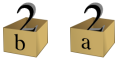
b is a second box, with a copy of integer 2. Box a has a separate
copy. Note how this is different to the final case we ended up for
Python above (b = a), there we have two names pointing to
the same value i.e. in Python, with integers, we do not copy the value
by assigning to another name, rather, we reference to it twice!
Nametag vs Box Semantics
WRITEME
Value, Variable, Assignment
A variable is a name that represents or refers to a value (an object
with some content) — variables names should be chosen appropriately,
matching whatever is semantically correct for the situation at hand.
The process of pointing a variable to a value is called assignment.
For example, the statement myvar = 42 assigns (using
=) the value 42 to the variable myvar.
Instead of saying pointing to, it is common to say that we are binding
the name myvar to the value (or rather object) 42 — in Python
everything is an object remember?
Assignments always go into the innermost scope. Also,
they do not copy data, rather, an assignment binds a name to an
object.
Assignment
We have just seen one above: myvar = 42. Assignment
statements modify namespaces, not objects. In other words, foo =
10 means that we are adding the name foo to our local
namespace, and making it refer to an integer object containing the
value 10. If the name is already present, the assignment replaces the
original name:
foo =
10
foo = 20
means that we are first adding the name foo to the local namespace,
and making it refer to an integer object containing the value 10. We
are then replacing the name, making it point to an integer object
containing the value 20. The original 10 object is not affected by
this operation, and it does not care. In contrast, if we do
foo = []
foo.append(1)
we are first adding the name foo to the local namespace, making it
refer to an empty list object. This modifies the namespace. We are
then calling a method on that object, telling it to append an integer
object to itself. This modifies the content/value of the list object,
but it does not touch the namespace, and it does not touch the integer
object.
Things like foo.attr and foo[index] are just syntactic sugar for
method calls. The first corresponds to __setattr__ and __getattr__,
the second to __setitem__ and __getitem__ (depending on which side of
the assignment they appear).
Chained Assignment
We can do it the unpythonic way first:
>>> bar = 5                                     # bind name bar to value 5
>>> foo = 5
>>> bar
5
>>> foo
5
>>> foo == bar                                  # equality check
True
>>> foo is bar                                  # identity check
True
>>> del bar                                     # remove binding
>>> del foo
>>> bar
Traceback (most recent call last):
  File "<input>", line 1, in <module>
NameError: name 'bar' is not defined
Now, the pythonic way:
>>> foo = bar = 5                               # chained assignment
>>> foo
5
>>> bar
5
>>> foo == bar
True
>>> foo is bar
True
Now, let us change the current value of foo, thus effectively binding
the name foo to another value:
>>> foo = foo + 1
>>> foo
6
>>> foo == bar
False
>>> foo is bar
False
>>>
Augmented Assignment
We can do
>>> somename = 10
>>> somename = somename + 1
>>> somename
11
>>>
or we can use an augmented assignment
>>> somename = 10         # new assignment rebinds the name somename to value 10 again
>>> somename += 1
>>> somename
11
>>>
Both are semantically equivalent and yield the same result. The latter
however is more pythonic and concise. Note that augmented assignments
are nothing specific to Python but rather many programming languages
have them.
Sequence Packing/Unpacking
This works for arbitrary iterables e.g. lists, strings, tuples, etc.
>>> mytuple = 4, 'foo', ['bar', 3, 'nose']      # sequence packing
>>> mytuple
(4, 'foo', ['bar', 3, 'nose'])
>>> x, y, z = mytuple                           # sequence unpacking
>>> x
4
>>> y
'foo'
>>> z
['bar', 3, 'nose']
>>> mytuple[2][1] == z[1]                       # evaluates to 3 == 3
True
>>>
While the above is probably known to most people, extended iterable
unpacking (introduced with PEP 3132) might not be:
>>> list(range(6))
[0, 1, 2, 3, 4, 5]
>>> x, *y, z = range(6)                         # *foo can be at any position e.g. middle
>>> x
0
>>> z
5
>>> y
[1, 2, 3, 4]
>>> type(y)
<class 'list'>                                  # not a tuple but a list
>>> *foo, baz = range(3)
>>> foo
[0, 1]
>>> baz
2
>>> *foo, baz, *bar = range(8)                  # there can only be one ;-]
  File "<input>", line 1
SyntaxError: two starred expressions in assignment
>>> foo = {}
>>> foo[0] = (1, 2)
>>> foo[1] = (3, 4, 5, 9)
>>> for a, (b, *c) in foo.items():
...     print(a, b, c)
...
...
0 1 [2]
1 3 [4, 5, 9]
>>>
Some might expect to receive a tuple when assigning to *foo (such as
with *args) but maybe it is worth noting that what we actually get is
a list.
Sequence unpacking is also useful when returning multiple values e.g.
if we wanted to choose a pythonic way of returning values from a
function, this is what we can do:
>>> import os
>>> filename, extension = os.path.splitext('picture.png')
>>> filename
'picture'
>>> extension
'.png'
>>>
Tuple Unpacking
A tuple is a sequence. Unpacking it in a pythonic manner also adheres
to the notion that tuples are not just read-only lists:
>>> connections = []
>>> connections.append(('1.1.1.1', 223))
>>> connections.append(('2.2.2.2', 12112))
>>> connections.append(('123.212.1.2', 42344))
>>> connections
[('1.1.1.1', 223), ('2.2.2.2', 12112), ('123.212.1.2', 42344)]
>>> type(connections)
<class 'list'>
>>> type(connections[0])
<class 'tuple'>
>>> for (ip_address, port) in connections:
...     if port > 1023:
...         print("Connection on IP {:>17} using port {:>5}.".format(ip_address, port))
...
...
...
Connection on IP           2.2.2.2 using port 12112.
Connection on IP       123.212.1.2 using port 42344.
>>>
Reading this code tells us that connections is a list containing
tuples of the form (ip_address, port). This is much clearer/pythonic
than using for item in connections and then poking inside item using
item[0] or similar techniques.
Mutable vs Immutable
Immutable objects cannot change their value/content and keep their ID
as mutable ones can — they cannot be modified in place as their
mutable counterparts. In other words, if we want to alter an immutable
object, we need to create a new/different one — the new one will have
a different ID. As a CPython implementation detail: id() returns the
memory address of the object.
Immutable objects play an important role in places where a constant
hash value is needed, for example as a key in a dictionary or member
of a set. To name a few immutable objects: numbers, strings, tuples,
frozensets, byte, None, etc. What all those have in common is that
they are Python built-in data structures.
It is fair to say that immutable datatypes can be thought of as the
basic building blocks used to assemble more complex datatypes e.g. if
we use a class to create ourselves a particular datatype used for our
individual web application, this class, or rather instances thereof,
would probably be mutable but some of its attributes might not be.
In a Nutshell
The majority of Python's built-in datatypes are immutable i.e. they
cannot change their value/content without changing their ID — they
cannot be modified in place as their mutable counterparts. Most custom
datatypes (e.g. a user-defined class) on the other hand are mutable
but might have attributes made of immutable built-in datatypes.
Equality vs Identity
is checks to see if two objects are actually one and the same object
whereas == checks if they are equal. For example, there
can be a case where two or more objects are equal but not identical:
>>> foo = bar = list(range(4))                  # two names binding to the same list object
>>> baz = list(range(4))                        # a third name binding to a second lists object
>>> foo
[0, 1, 2, 3]
>>> bar
[0, 1, 2, 3]
>>> baz
[0, 1, 2, 3]
>>> id(foo)
39291432
>>> id(bar)
39291432
>>> id(baz)
40455344
>>> foo == bar == baz                           # equality check
True
>>> foo is bar is baz                           # identity check
False
>>> foo is bar
True
>>> foo is baz
False
>>> foo is bar is not baz
True
>>>
As can be see, foo and bar are identical but not baz — we are dealing
with two objects thus two IDs. foo and bar are two different names
binding to the same value (or rather object) whereas baz is not just a
different name but also binds to a different object.
A prominent example of when it actually makes quite a difference
whether we check for equality or identity is with None.
Callable
A Callable is an abstract form of a function respectively an arbitrary
Python object that mimics the behavior of a function in that it can
be called.
In other words, any callable object (e.g. user-defined functions,
built-in functions, methods of built-in objects, class objects,
methods of class instances, and all objects having a __call__()
method) that has an interface which defines that an object acts like
as if were a function is said to be callable. Like an ordinary
function, a callable may take parameters and it may also return
something.
Many kinds of objects in Python are callable, and they can serve many
different purposes:
- Functions are callable, and they may carry along a closure from an
outer function
- Classes are callable, and calling a class gets us an instance of
that class
- Methods are callable, for function-like behavior specifically
pertaining to an instance
- Class methods and static methods are callable, for method-like
functionality when the functionality pertains to a whole class in
some sense (static method's usefulness is dubious, since a class
method could do just as well
- Generators are callable, and calling a generator gets us an
iterator object
- Finally, we can write a class whose instances are callable. This is
often the simplest way to have calls that update an instance's
state as well as depend on it (though a function with a suitable
closure, and a bound method, offer alternatives, a callable
instance is the one way to go when we need to perform both calling
and some other specific operation on the same object — for
example, an object we want to be able to call but also apply
indexing to had better be an instance of a class that is both
callable and indexable).
Examples
The callable() built-in function from Python 2 was resurrected with
Python 3.2. It provides a concise and more readable alternative to
using an abstract superclass in an expression like isinstance(x,
collections.Callable) and is thus considered the pythonic way of
checking whether or not something is callable:
>>> def foo():
...     pass
...
...
>>> callable(foo)
True
>>> callable(39)
False
>>> callable(max)
True
>>> max(3, 5, 88)
88
>>> callable(None)
False
>>>
Making something callable
hashable
WRITEME
First-class Object
WRITEME
Object-Oriented Relationships
This subsection explains the type-instance and supertype-subtype
relationships, and can be safely skipped if the reader is already
familiar with these OOP concepts. Skimming over the rules below might
be useful though.
Meet Squasher

This is Squasher. Squasher is a super-smart Python, so smart in fact
that he is going to help me explain object-oriented relationships...
Types of Relationships
While there are many different objects, there are basically only two
kinds of relationships:
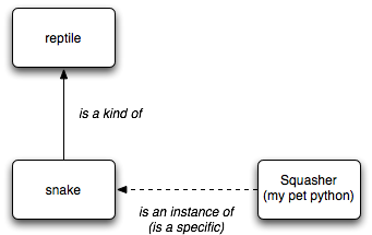
- is a kind of
-
(solid line) — known to the OOP folks as specialization, this
relationship exists between two objects when one (the
subclass/subtype) is a specialized version of the other (the
superclass). A snake is a kind of reptile — it has all the
characteristics of a reptile plus some specific characteristics which
specifically identify it as a snake. Terms used: subclass of,
superclass of and superclass-subclass.
- is an instance of
-
(dashed line) — also known as instantiation, this relationship exists
between two objects when one (the instance) is a concrete example of
what the other specifies (the type). Squasher is an instance of a
snake — snake is the blueprint used to build Squasher (and possibly
many more other individual snakes). Terms used: instance of, type of,
type-instance and class-instance.
Beware of Ambiguity
Note the ambiguity in plain English: The term is a is used for both of
the above relationships i.e. people tend to say Squasher is a snake
and snake is a reptile.
That is wrong because it is ambiguous, it leads to confusion and thus
mistakes. In order to avoid ambiguity and therefore be able to
properly distinguish both cases, the terms outlined above should be
used.
Properties of Relationships
It is useful at this point to note the following (independent)
properties of relationships:
- Dashed Arrow Up Rule
-
If X is an instance of A, and A is a subclass of B, then X is an
instance of B as well.
- Dashed Arrow Down Rule
-
If B is an instance of M, and A is a subclass of B, then A is an
instance of M as well.
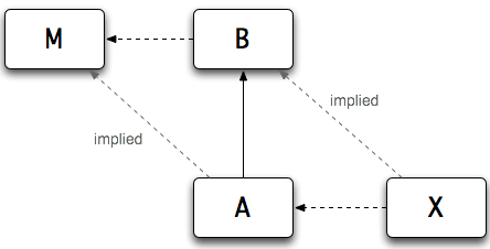
In other words, the head end of a dashed arrow can move up a solid
arrow, and the tail end can move down. These properties can be
directly derived from the definition of the is a kind of
(superclass-subclass) relationship.
Using the Dashed Arrow Up Rule on our reptile/snake/Squasher example
from above we can now conclude that 1) Squasher is an instance of
snake (the type of Squasher is snake) and 2) Squasher is an instance
of reptile (the type of Squasher is reptile).... Hmm... What?...
Squasher has two types? Well, no...
Earlier we said that every object has exactly one type. So how come
Squasher seems to have two? Note that although both statements are
correct, one is more correct (and in fact subsumes the other). In
other words:
squasher.__class__ is Snake — the __class__ attribute points to
the type of an object.- both
isinstance(squasher, Snake) and isinstance(squasher, Reptile)
are true... Dashed Arrow Up Rule.
>>> class Reptile():                            # real code would have docstrings
...     pass
...
...
>>> class Snake(Reptile):                       # subclassing Reptile
...     pass
...
...
>>> squasher = Snake()                          # instantiating a snake; moment of birth for Squasher
>>> squasher.__class__
<class '__main__.Snake'>                        # Squasher's type is Snake
>>> isinstance(squasher, Snake)
True
>>> isinstance(squasher, Reptile)
True                                            # Dashed Arrow Up Rule
>>> issubclass(Snake, Reptile)
True
>>> Reptile.__bases__
(<class 'object'>,)                             # huh? more on that later...
>>> Snake.__bases__
(<class '__main__.Reptile'>,)                   # Snake is a kind of Reptile
>>>
A similar rules exists for the is a kind of (superclass-subclass)
relationship:
- Combine Solid Arrows Rule
-
If A is a subclass of B, and B is a subclass of C, then A is a
subclass of C as well.
Now assume we had subclassed Reptile from an Animal class, thus we
could say: A snake is a kind of reptile, and a reptile is a kind of
animal, therefore a snake is a kind of animal:
Snake.__bases__ is Reptile. Nothing changed. But, Reptile.__bases__
would now be Animal instead of object. Note that it is possible for
an object to have more than one superclass in case of
multiple-inheritance.- Both
issubclass(Snake, Reptile) and issubclass(Snake, Animal) are
true.
Object System
This subsection will help us understand how objects in Python are
created, when this happens and why.
Basic Concepts
Now, after some little detour to object-oriented relationships and
after cementing the notion of key-facts about objects into our brains,
we are now ready to take a detailed look at objects in Python, what
they are, why they are useful and why they behave the way the do.
So what exactly is a Python object? An object is an axiom in our
system i.e. it is the notion of some entity, the most basic building
block used to build everything else. We define an object by saying it
has:
- Identity i.e. given two names we can say for sure whether or not
they refer to one and the same object.
- Zero or more names — one might think an object has a name but the
name is not really part of the object itself but rather exists
outside of the object in a namespace or as an attribute of another
object.
- A value which may include a bunch of attributes i.e. we can reach
other objects through
objectname.attributename.
- A type, of which we already know by now that
every object has exactly one type. For instance, the object
2 has a
type int and the object "joe" has a type string.
- One or more superclasses. The type and superclasses are important
because they define special relationships an object has with other
objects — types and superclasses of objects are just other objects.
- Each object also has a specific location in memory that we can find
by calling the id() function.
Example
Even a simple object such as the number 2 has a lot more to it than
meets the eye:
 1  >>> foo = 2
 2  >>> type(foo)
 3  <class 'int'>
 4  >>> type(type(foo))
 5  <class 'type'>
 6  >>> type(foo).__bases__
 7  (<class 'object'>,)
 8  >>> dir(foo)
 9  ['__abs__',
10   '__add__',
11   '__and__',
12   '__bool__',
13
14
15  [skipping a lot of lines...]
16
17
18   'conjugate',
19   'denominator',
20   'from_bytes',
21   'imag',
22   'numerator',
23   'real',
24   'to_bytes']
25  >>>
In line 1 we give an integer the name foo in the current namespace.
The type of this object is int, <class 'int'> the
representation of its type. As can be seen in line 5, the object used
to represent the type of the object of type int is itself an object,
of type type this time.
The __bases__ attribute of <class 'int'> is a tuple
containing an object called <class 'object'>. In lines 8
to 24 we list all of the foo object's attributes. One might ask what
are those? Where do they come from? Well, as we already know ... in
Python everything is an object!
Of course, the built-in int is an object too...This does not mean
that just the numbers such as 2 and 77 are objects (which they are)
but also that there is another object called int that is sitting in
memory right beside the actual integers. In fact all integer objects
are pointing to this int object using their __class__ attribute saying
that guy knows me all about me. Calling type() on an object just
returns the value of the __class__ attribute.
Any class we define is an object, and of course, instances of those
classes are objects as well. Even the functions and methods we define
are objects. Yet, as we will see, not all objects are made equal.
Clean Slate
We are now going to build the Python object system from scratch. Let
us begin at the beginning... with a clean slate:

One might be wondering why a clean slate has two grey lines running
vertically through it. All will be revealed later. For now this will
help distinguish a slate from other figures. On this clean slate, we
will gradually put different objects, and draw various relationships,
until it is left looking quite full.
At this point, it helps if any preconceived object oriented notions of
classes and objects are set aside, and everything is perceived in
terms of objects and relationships.
Relationships
As we introduce many different objects, we use
two kinds of relationships to connect them. These are the is a kind of
(subclass-superclass) relationship and the is an instance of
(type-instance) relationship.
Add the Objects
We are now going to start looking at the object system, bottom-up,
i.e. we start with the two most basic objects:
type and object
We examine two objects: <class 'object'> and <class
'type'>.
1 >>> object
2 <class 'object'>
3 >>> type
4 <class 'type'>
5 >>> type(object)
6 <class 'type'>
7 >>> type(type)
8 <class 'type'>
9 >>> object.__class__
10 <class 'type'>
11 >>> object.__bases__
12 ()
13 >>> type.__class__
14 <class 'type'>
15 >>> type.__bases__
16 (<class 'object'>,)
17 >>>
Lines 1 to 8 show the names respectively representations of the two
most basic objects in Python, object and type. The type() function was
introduced as a way to find the type of an object by looking at its
__class__ attribute. The __class__ attribute in fact is both, an
object itself, and a way to get the type of another object.
In line 5 we start exploring object. The type of object is type. In
line 9 we also use the __class__ attribute and verify it is the same
as calling type() in line 5.
By exploring type we find out that the type of type is type. Huh? The
__bases__ of object type in lines 13 and 14 yield the same result.
What is going on here? Let us make use of our so far clean slate and
draw what we have seen:
- type is now class
-
Note that all pictures still show e.g.
<type 'object'>
instead of <class 'object'> i.e. type instead of class.
The latter one is the now (Python 3 onwards) correct representations
we get when we use type() or directly look at an objects's __class__
attribute.
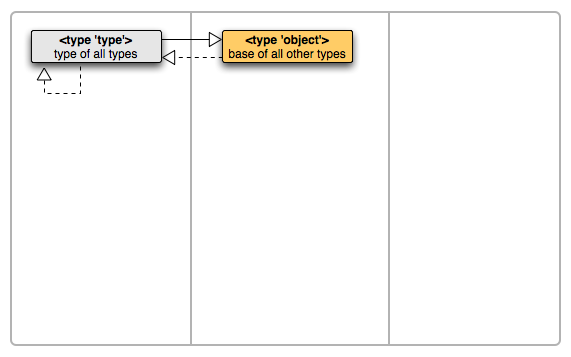
These two objects, type and object, are the two most basic objects in
Python. We might as well have introduced them one at a time but that
would lead to the chicken and egg problem... which to introduce
first? These two objects are interdependent i.e. they cannot stand on
their own since they are defined in terms of each other.
Let us continue with our explorations:
1 >>> isinstance(object, object)
2 True
3 >>> isinstance(type, object)
4 True
5 >>>
In lines 1 and 2 we can see the Dashed Arrow Up Rule in action again.
Since <class 'type'> is a subclass of <class
'object'>, instances of <class 'type'> are
instances of <class 'object'> as well.
Lines 3 and 4 show applying both, the Dashed Arrow Up Rule and the
Dashed Arrow Down Rule which effectively reverses the direction of the
dashed arrow.
Type Object
Now for a new concept... type objects. Both of the objects we
introduced so far (type, object) are type objects. Type objects share
the following characteristics:
- They are used to represent abstract data types in programs. For
example, a user defined object called
User might represent all
users in a system, another one called int might represent all
integers.
- They can be subclassed (is a kind of relationship). This means we
can create a new object that is somewhat similar to an existing
type objects. The existing type objects become
superclasses/supertypes for the new one.
- They can be instantiated. This means we can create a new object
that is an instance of the existing type object. The existing type
object becomes the
__class__ attribute for the new object.
- The type of any type object is
<class
'type'>
.
Since the introduction of new-style classes, types and classes are
really the same in Python. Thus it is no wonder that the type()
function and the __class__ attribute gets us the same results.
Before new-style classes were introduced types and classes had their
differences. The term class was traditionally used to refer to a class
created by the class statement. Built-in types (such as int and
string) are not usually referred to as classes, but that is more of a
convention and in reality type, type object and class is the same
thing — since Python 2.3 the terms type, type object and class are
all equivalent.
Type/Non-Type Types
Types and, for lack of a better word, non-types are both objects but
only types can have subclasses. Non-types are concrete values so it
does not make sense for another object to be a subclass of a non-type.
Three good examples of objects that are non-types are the integer 2,
the list foo (e.g. made by issuing foo = [1, 4, 3]) and
the string Hello World.
- Type vs Non-type
-
If an object is an instance of
<class 'type'>, it is a
type, a non-type otherwise.
We can verify that this rule is true for all objects we have come
across so far, including <class 'type'> which is an
instance of itself. Let us summarize:
<class 'object'> is an instance of <class
'type'>.<class 'object'> is a subclass of no object. In other
words: it has no superclasses/supertypes. It is the most basic
object, used to build all other objects from.<class 'type'> is an instance of itself.<class 'type'> is a subclass of <class
'object'>.- There are only two kinds of objects in Python —
types and
non-types. Non-types can be called instances, but that term could
also refer to a type, since a type is always an instance of another
type. Types can also be called classes.
Note that we are drawing arrows on our slate for only the direct
relationships, not the implied ones i.e. only if one object is
another's __class__ attribute or is listed in the other's __bases__
attribute (which we know by now is a tuple). This makes economic use
of the slate and our mental capacity.
Built-in Types
We already scratched the surface of built-in types earlier. Now we are
going to give it a more detailed look. Python does not ship with only
two objects, oh no, the two basic types (type, object) come with a
whole bunch of children.
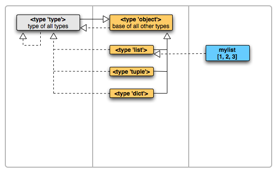
This diagram shows a few built-in types. Let us have a closer look at
them:
1 >>> list
2 <class 'list'>
3 >>> list.__class__
4 <class 'type'>
5 >>> list.__bases__
6 (<class 'object'>,)
7 >>> tuple.__class__
8 <class 'type'>
9 >>> tuple.__bases__
10 (<class 'object'>,)
11 >>> dict.__class__
12 <class 'type'>
13 >>> dict.__bases__
14 (<class 'object'>,) # object is the supertype/superclass of all objects
15 >>> mylist = [1, 2, 3] # encoding an objects type into its name is unpythonic
16 >>> mylist.__class__
17 <class 'list'>
18 >>>
Line 2 shows the representation of the type of the built-in list type
object. We also know that behind an object's __class__ attribute we
find another object, the actual type object of the object that tells
us anything about the type of an object.
In line 6 we can see that the built-in list type is subclassed from
the built-in object type. No surprise here, we know that object is the
supertype/superclass of any other type in Python.
All things just said about list are true for tuple and dict as well.
In line 15 we instantiate a non-type type (is an instance of
relationship), same thing we did with Squasher when we issued
squasher = Snake(). Line 17, another no-brainer, the type
object attached to the __class__ attribute of our mylist instance is
the type object representing the built-in type list.
Of course, when we create a tuple or a dictionary, they are instances
of their respective built-in types as well.
Last but not least, how can we create an instance of mylist? Well, we
cannot, mylist is a concrete value thus it is a non-type therefore it
cannot be instantiated. Also, with regards to mylist, it is usually
not considered pythonic to encode an objects type into its name. We
have done it in this section to make things a bit easier to understand
as usually people reading through this section might already struggle
to comprehend all knowledge presented.
New Objects by Subclassing
The built-in types are, well, built into Python. They are there when
we start Python, and remain their after we finish. However, how can we
create new types? New types cannot pop out of thin air, rather they
have to be built using existing ones.
>>> class C: # implicitly subclassed from object
... pass
...
...
>>> class D:
... pass
...
...
>>> class E(C, D):
... pass
...
...
>>> C.__class__
<class 'type'> # Dashed Arrow Down Rule
>>> D.__class__
<class 'type'>
>>> E.__class__
<class 'type'>
>>> C.__bases__
(<class 'object'>,)
>>> D.__bases__
(<class 'object'>,)
>>> E.__bases__
(<class '__main__.C'>, <class '__main__.D'>)
>>>
At first we create two new types (C and D) by subclassing object —
the class keyword tells Python to create a new type by subclassing an
existing type. We also create a new type E that is not subclassed from
object but from C and D. Most built-in types can be subclassed (but
not all).
Subclassing built-in Types
Subclassing built-in types is straightforward, actually we have been
doing it all along whenever we subclassed object before. However,
there are some built-in types (e.g. function) which cannot be
subclassed (yet). Let us have a look at subclassing two of the most
notorious built-in types, list and tuple:
1 >>> class Foo(list):
2 ... def append(self, item): # overrides append from the built-in list type
3 ... list.append(self, int(item))
4 ...
5 ...
6 ...
7 >>> bar = Foo()
8 >>> type(bar)
9 <class '__main__.Foo'>
10 >>> Foo.__bases__
11 (<class 'list'>,)
12 >>> bar
13 []
14 >>> bar.append(3)
15 >>> bar
16 [3]
17 >>> bar.append(2.432)
18 >>> bar
19 [3, 2]
20 >>> len(bar)
21 2
22 >>> bar[1] = 2.432
23 >>> bar
24 [3, 2.432]
25 >>> bar.color = "blue"
26 >>> bar
27 [3, 2.432]
28 >>> bar.color
29 'blue'
30 >>>
In lines 2 to 3 we override the append method of the built-in list
type so that appended items are always casted to int e.g. lines 17
to 19. What we can also see from line 3 is that overriding append
basically works like an unbound method in that we explicitly pass the
instance as its first argument. Line 20 shows that len() on our list
subclass/subtype works just like on any instance of type list as well.
The other interesting bit is with lines 22 to 24. As we can see,
assignments to a particular index position of our list instance bar do
not go trough our version of append (lines 2 and 3), the one used to
override append in the original list type which we subclassed from.
In order to have the same casting in place for assignments as well we
would have to define the special method __setitem__() in our Foo class
to massage such data. The call would then be to
list.__setitem__(self, item).
Because the list type (and therefore any of its subclasses/subtypes)
has a __dict__ we can set arbitrary attributes and assign values to
the dictionaries key e.g. the value blue to the key color. In some
cases however having a __dict__ might not be favorable because of the
implicit amount of space that is needed. We might thus decide to give
our subclasses/subtypes a __slots__ attribute which can help a great
deal in cases where we have a very high number of instances.
Customizing the instantiation and creation process...
Another way of creating a list subclass/subtype is by customizing its
instantiation process. Instantiating a list subclass/subtype works
just like instantiating any other type works which is by calling
list([1, 2, 3]) or, even better, just [1, 2, 3].
The way we customize the instantiation/creation process of a list
subclass/subtype is by having the special method __init__() overridden
in the subclass/subtype. The __init__() special method of the built-in
list class/type accepts any iterable types and uses them to initialize
a list — the subclass/subtype has to do the same.
Tuples are immutable and different from lists such that once a tuple
instance is created, it cannot be changed (modified in place) anymore.
In general, every time a new instance of some class/type is created,
two special methods are called —
first __new__() then __init__().
The instance of a type already exists when __init__() is called on it
—
__init__() is a bound method i.e. the instance is passed as
implicit first argument, named self by convention.
The __new__() special method is a class method that is called when we
want to create a new instance of some class/type. It is passed the
class/type itself as implicit first argument (named cls by
convention), and passed through other initial arguments (similar to
__init__()). Overriding __new__() is often used in order to customize
immutable types like a for example tuples.
1 >>> class Foo(list): # real code would have docstrings
2 ... def __init__(self, itr):
3 ... list.__init__(self, [int(item) for item in itr])
4 ...
5 ...
6 ...
7 >>> class Bar(tuple):
8 ... def __new__(cls, itr):
9 ... seq = [int(item) for item in itr]
10 ... return tuple.__new__(cls, seq)
11 ...
12 ...
13 ...
14 >>> bazbar = Foo() # we need to supply an iterable
15 Traceback (most recent call last):
16 File "<input>", line 1, in <module>
17 TypeError: __init__() takes exactly 2 arguments (1 given)
18 >>> bazbar = Foo([1, 32.243, 111.2])
19 >>> bazbar
20 [1, 32, 111]
21 >>> type(bazbar)
22 <class '__main__.Foo'>
23 >>> bazbar.__class__
24 <class '__main__.Foo'>
25 >>> Foo.__bases__
26 (<class 'list'>,) # Foo is a list subclass/subtype
27 >>> foobaz = Bar()
28 Traceback (most recent call last):
29 File "<input>", line 1, in <module>
30 TypeError: __new__() takes exactly 2 arguments (1 given)
31 >>> foobaz = Bar([2.3, 3.42433, 4])
32 >>> foobaz
33 (2, 3, 4)
34 >>> Bar.__bases__
35 (<class 'tuple'>,) # Bar is a tuple subclass/subtype
36 >>> type(foobaz)
37 <class '__main__.Bar'>
38 >>> foobaz[1] = 3.23 # tuples are immutable
39 Traceback (most recent call last):
40 File "<input>", line 1, in <module>
41 TypeError: 'Bar' object does not support item assignment
42 >>> foobaz[1]
43 3
44 >>> bazbar[1]
45 32
46 >>> bazbar[1] = 4.32 # lists are mutable
47 >>> bazbar
48 [1, 4.32, 111]
49 >>>
The difference of customizing the instantiation/creation process
depending on whether or not we subclass immutable or mutable types can
be seen from lines 1 to 13. For immutable types we need to override
__new__() whereas for mutable types overriding __init__() is all we
need to do.
In both cases we take an iterable as second argument and cast its
items to int using a list comprehension. A __new__() special method
should always have an explicit return statement that should return an
instance of the type.
Note that the __new__() special method is not special to immutable
types, it is used for all types. It is also converted to a class
method automatically by Python.
New Objects by Instantiation
Subclassing is only half the story of new types...
>>> obj = object()
>>> type(obj)
<class
'object'>
>>> cobj = C()
>>> type(cobj)
<class '__main__.C'>
>>> class FooBar(list):
... pass
...
...
>>> FooBar.__bases__
(<class 'list'>,)
>>> foo = FooBar()
>>> type(foo)
<class '__main__.FooBar'>
>>> isinstance(foo, list) # Dashed Arrow Up Rule
True
>>>
The call operator (()) creates a new object by instantiating an
existing one. The existing object must be a type rather than a
non-type for this to work. Depending on the type, the call operator
might accept arguments as well. For many built-in types there is a
pythonic way of creating new objects. For example, square brackets
([]) create an instance of type list. A numeric literal creates an
instance of int.
Of course, we can subclass list, instantiate our new type and check
whether or not it is actually an instance of the built-in type list
... yet another example of the Dashed Arrow Up Rule... After the
above exercise, our slate looks quite full:
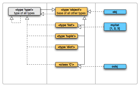
Note that by implicitly subclassing object, the C and D types
automatically become an instance of type (Dashed Arrow Down Rule). As
we can see e.g. C.__class__ verifies this. Why this happens is
explained below.
Notes on Instantiation
How does Python really create a new object?
-
Internally, when Python creates a new object, it always uses a type
and creates an instance of that particular type. Specifically it uses
the
__new__() and __init__() special methods of the particular type.
In a sense, the type serves as a factory that can churn out new
objects of a particular type. In other words, the manufactured objects
will point to the same type object which the one used to create them
points to. This is why every object has a type.
When using instantiation, we specify the type, but how does Python
know which type to use when we use subclassing?
-
It looks at the superclass, and uses its type as the type for the new
object. A little thought reveals that under most circumstances, any
subclasses of
object (and their subclasses, and so on) will have type
as their type. Advanced Material Ahead
Can we instead specify a particular type to use?
-
Yes, by using the __metaclass__ class attribute.
Can we use any type for an object's __metaclass__ class attribute?
-
No. It must be a subtype/subclass of the supertype's/superclass's
type.
What if we have multiple supertypes/superclasses, and do not specify a
__metaclass__ class attribute, which type will be used?
-
This depends on whether or not Python can figure out which one to use.
If all the superclasses have the same type, for example, then their
type will be used. If they have different types unrelated types, then
Python cannot figure out which type object to use. In this case
specifying a
__metaclass__ class attribute is required, and this
__metaclass__ class attribute must be a subclass/subtype of each of
the types of each superclasses.
Wrap Up
We ended up with a comprehensive map of Python's object system. Here
we also unravel the mystery of the vertical grey lines. They just
segregate objects into three spaces based on what the common man calls
them — metaclasses, classes, and instances.
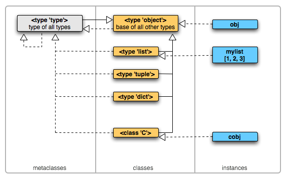
- Dashed lines cross spacial boundaries i.e. go from object to
meta-object. Only exception is
<class 'type'> (which
is good, otherwise we would need another space to the left of it,
and another, and another...).
- Solid lines do not cross space boundaries. Again,
<class
'type'> to <class 'object'> is an exception.
- Solid lines are not allowed in the rightmost space. These
objects/types are too concrete to be subclassed.
- Dashed line arrow heads are not allowed into rightmost space.
These objects/types are too concrete to be instantiated.
- The left two spaces contain types. The rightmost space contains
non-types.
- If we created a new object/type by subclassing
<class
'type'> it would be in the leftmost space, and would also
be both, a subclass and instance of <class 'type'>.
It is also worth noting that <class 'type'> is indeed the
supertype of all type objects, and <class 'object'> the
supertype/superclass of all types (except itself).
Summary
There are two kinds of objects in Python:
- Type objects/types, these can create instances and can be
subclassed.
- Non-type objects/types, these cannot create instances and they
cannot be subclassed.
type and object are the two most basic objects of the system.objectname.__class__ exists for every object and points to another
object, the type object for the particular supertype/superclass of
the object which has the name objectname bound to it.objectname.__bases__ is a tuple that exists for every type object
containing its supertype(s)/superclasse(es). It is empty only for
object.- To create a new object using subclassing, we use the
class keyword
and specify the supertype(s)/superclass(es) and, optionally, the
type of the new object. This always creates a new type object/type.
- To create a new object using instantiation, we use the call
operator (
()) on the type object we want to instantiate from. This
may create a type or a non-type object/type, depending on which
type object was used.
- Some non-type objects can be created using a
pythonic way of creating new objects. For example,
baz = [1,
8, 3]
creates a list instance (baz) of the built-in type
list.
- Internally, Python always uses a type object to create a new
object. The new object created is an instance of the type object
used. Python determines the type object from a class statement by
looking at the supertype(s)/superclass(es) specified, and finding
their types.
issubclass(A, B) is testing for the is a kind of
(superclass-subclass) relationship and returns True if:
B is in A.__bases__ orissubclass(Z, B) is true for any Z in A.__bases__. isinstance(A, B) is testing for the is an instance of relationship
and returns True if:
B is A.__class__ orissubclass(A.__class__, B) is true.
Attribute
Next to understanding iterators, descriptors, decorators and how the
object system in Python works, understanding what attributes are, how
they are accessed and what intrinsic semantics go along with doing so,
is probably the most important thing to know for any Pythoneer out
there.
A value associated with an object which is referenced by name using
dotted expressions. For example, if object foo had an attribute attr
it would be referenced as foo.attr... On the next level down the
rabbit hole we could say that in fact an attribute is a way to get
from one object to another (because attr on object foo simply is yet
another object).
When we apply the power of the almighty dotted expression
(objectname.attributename) we end up with the handle to another
object. And, of course, we cannot just lookup attributes but we can
also create attributes, by assignment: objectname.attributename
= someobject.
Attribute Access
Which object does an attribute access return though? Where does the
object set as an attribute end up? What are the ties between attribute
access and inheritance? And most importantly, what exactly does
attribute access mean? Let us have a look...
>>> class Ding:                 # real code would have docstrings
...     pass
...
...
>>> dong = Ding()
>>> dong.foo = 2                # setting an attribute by assignment
>>> dong.foo                    # attribute reference
2
>>> del dong.foo                # attribute deletion
>>>
An attribute can be referenced, assigned to or deleted. Any of these
or any combination thereof is what we call attribute access. What
exactly happens during attribute access is explained next.
Examples of Attribute Access
Let us start with the simplest of attribute access types, referencing
an attribute. An attribute reference is an expression of the form
foo.name where foo can be any valid Python expression and name is an
identifier called the attribute name.
- Many kinds of Python objects have attributes but an attribute
reference shows different semantics depending on whether or not
the attribute is referenced from a class/type or some instance
thereof.
- Also, attributes might be callable e.g. an object might have a
method as one of its attributes. Again, different semantics are
the result.
- Another thing greatly influencing how attribute access is done
depends on the type of attribute access (setting, referencing,
deleting). For example, setting an attribute follows a different
algorithm compared to referencing it, thus two very different
semantics can be observed.
We can already see that there are quite a few combinations with
regards to attribute access depending on
- which of the three attribute access types we do as well as
- whether we do it on a class/type or an instance thereof and
- whether or not the attribute is callable or not
While we now know that the algorithm used to figure out what to do
when an attribute access happens, let it be known that we can of
course entirely customize attribute access. However, let us not get
ahead of ourselves and start with the basics:
>>> class Foo:                                          # real code would have docstrings
...     baz = 23
...     bar = 45
...     def faz(self):
...         print("Method faz in class Foo.")
...
...     def foz(self):
...         print("Method foz in class Foo.")
...
...
...
>>> class Rab(Foo):                                     # subclassing Foo
...     bar = 89                                        # overriding bar
...     fuz = 32
...     noz = 314
...     def foz(self):                                  # overriding foz
...         print("Method foz in class Rab.")
...
...     def sna(self):
...         print("Method sna in class Rab.")
...
...
...
>>> fux = Rab()
>>> fux.noz = 22                                        # setting attributes on the instance will
>>> fux.niz = 42
>>> Rab.__name__
'Rab'
>>> del Rab.__name__
Traceback (most recent call last):
  File "<input>", line 1, in <module>
TypeError: can't delete Rab.__name__
>>> Rab.__bases__
(<class '__main__.Foo'>,)
>>> fux.__class__
<class '__main__.Rab'>
>>> type(fux)
<class '__main__.Rab'>
>>> Rab.__dict__
dict_proxy({'__module__': '__main__', 'bar': 89, 'noz': 314,
'sna': <function sna at 0x1adb1e8>, '__getattribute__': <slot
 wrapper '__getattribute__' of 'object' objects>, 'fuz': 32,
'__doc__': None, 'foz': <function foz at 0x1adb7c0>})
>>> fux.__dict__
{'niz': 42, 'noz': 22}                                  # put them into __dict__ on the instance
>>> dir(fux)
['__class__',                                           # attributes automatically set by Python
 '__delattr__',
 '__dict__',
 '__doc__',
 '__eq__',
 '__format__',
 '__ge__',
 '__getattribute__',
 '__gt__',
 '__hash__',
 '__init__',
 '__le__',
 '__lt__',
 '__module__',
 '__ne__',
 '__new__',
 '__reduce__',
 '__reduce_ex__',
 '__repr__',
 '__setattr__',
 '__sizeof__',
 '__str__',
 '__subclasshook__',
 '__weakref__',
 'bar',                                                 # attributes set by us
 'baz',
 'faz',
 'foz',                                                 # a method is an attribute too...
 'fuz',
 'niz',
 'noz',
 'sna']
>>> Rab.foz
<function foz at 0x1aec160>
>>> Rab.__dict__['foz']
<function foz at 0x1aec160>
>>> fux.foz                                             #... a so-called bound method
<bound method Rab.foz of <__main__.Rab object at 0x1b7fe90>>
>>> fux.foz()
Method foz in class Rab.
>>>
We create two classes/types, Foo and Rab where Rab is a
subclass/subtype of Foo. Then we override a few attributes on Rab,
instantiate an instance of Rab called fux and set a few more
attributes (noz and niz) on this instance. Note that in Python we can
shadow/override any type of attribute, whether it is a callable (e.g.
method) or just a simple literal, it does not make a difference.
It is worth nothing that every class/type has a few special attributes
such as __name__, __class__, __dict__, etc. As can be seen, we cannot
unbind them (del statement) but we can rebind them.
One special attribute that is of special interest to us is __dict__.
__dict__ is a dictionary containing the majority of a class's or
instance's attributes except for special ones such as mentioned
earlier (e.g. __name__). As can be seen, there is a difference whether
or not we look at the class's __dict__ or the instance's __dict__. The
latter only contains attributes that were explicitly set by us (niz
and noz).
Using the dir() function on the fux instance gives us all its
attributes (as opposed to using fux.__dict__), including its class
attributes and also, recursively up the inheritance chain, all the
attributes of all of its class's superclass(es)/supertype(s). Without
arguments dir() just returns the list of names in the current local
scope.
Then, finally, a look at a method and as can be seen, a method really
is nothing special but just yet another attribute and depending on
where/how it is accessed it is bound/unbound etc.
It is now time to have a look at how exactly an attribute lookup
works and how it differs on whether or not we start out on a
class/type itself or an instance thereof.
Getting an Attribute from a Class
Using Rab.name in order to refer to an attribute on a class involves a
two step process:
- name is a key in __dict__: When
name is a key in Rab.__dict__ then
Rab.name fetches the associated value val from
Rab.__dict__['name'].
- If this value
val is a descriptor (i.e. type(val) has a
__get__() special method) the value of Rab.name is the result of
calling type(val).__get__(val, None, Rab).
- Otherwise, if
val is not a descriptor, the result is val.
- name is NOT a key in __dict__: When
name is not a key in
Rab.__dict__, Rab.name delegates the attribute lookup to the
superclass(es)/supertype(s) of Rab (Foo in our case). The way this
works is basically by starting at Rab, then Python moves up the
inheritance chain and tries the name lookup from step 1 on every
class/type it encounters along its way up the inheritance chain
(see MRO (Method Resolution Order)) until it finds the name name
is a key in the current's class/type __dict__. It then proceeds as
described in step 1.
Getting an Attribute from an Instance
When we do fux.name we reference an attribute on the instance fux of
class/type Rab. In this case the lookup process is as follows:
- When
name is found in Rab (or some class/type higher up in the
inheritance chain) as the name of an shadowing/overriding
descriptor val, then the value of Rab.name is the result of
calling type(val).__get__(val, fux, Rab) i.e. we end up with a
call to the shadowing/overriding descriptor and provide to it the
instance on which the call originated on (fux), the instance's
class/type (Rab) and the value val (the actual descriptor).
- Otherwise, if
name is a key in fux.__dict__ then fux.name fetches
and returns its value at fux.__dict__['name'].
- Otherwise,
fux.name delegates the lookup to the class/type of fux
(according to the two-step lookup process outlined for
getting an attribute from a class). If val is found to be a
descriptor then we again end up with type(val).__get__(val, fux,
Rab). If on the other hand val is not a descriptor then the
overall result of the attribute lookup on the class is val.
Examples of Attribute access on Instances - non-callable Attributes:
>>> fux.__dict__
{'niz': 42, 'noz': 22}                          # niz and noz are keys in fux's __dict__
>>> fux.noz
22
>>> fux.niz
42
>>>
The two attributes niz and noz are so-called instance variables on
instance fux. The lookup process succeeds at step 2 of the instance
lookup process since no shadowing/overriding descriptors are involved
(step 1) and both attributes are keys in the __dict__ dictionary on
instance fux.
>>> fux.fuz
32
>>> fux.__class__.__dict__['fuz']               # semantically equivalent to ...
32
>>> Rab.__dict__['fuz']                         #... this one as can be seen below (same object)
32
>>> fux.__class__.__dict__['fuz'] is Rab.__dict__['fuz']
True
>>>
If we lookup the fuz attribute — a class/type variable — on instance
fux of the Rab class/type then we need to proceed to step 3 of the
instance lookup process and from there onto step 1 of the class/type
lookup process where it succeeds because fuz is a key in the
Rab.__dict__ dictionary, as can be seen above.
We can also see that there is more than one way to reference the fuz
object depending on which object we start from i.e. the instance or
the class object — in the end we arrive at the same object as the
identity check confirms.
>>> fux.baz
23
>>> Foo.__dict__['baz']                         # semantically equivalent to ...
23
>>> fux.__class__.__bases__[0].__dict__['baz']  #... this one as can be seen below (same object)
23
>>> Foo.__dict__['baz'] is fux.__class__.__bases__[0].__dict__['baz']
True
>>>
baz is a class/type variable on Foo, therefore, if we lookup the baz
attribute on instance fux of the Rab subclass/subtype of Foo, then we
need to proceed to step 3 of the instance lookup process first and
from there onto step 2 of the class lookup process before we again
arrive at step 1 of the class lookup process (after we moved up the
inheritance chain from Rab to Foo) where it succeeds because baz is a
key in Foo.__dict__.
Examples of Attribute access on Instances - callable Attributes:
>>> fux.sna
<bound method Rab.sna of <__main__.Rab object at 0x1b7fc50>>
>>> Rab.__dict__['sna'].__get__(fux, Rab)
<bound method Rab.sna of <__main__.Rab object at 0x1b7fc50>>
>>> Rab.sna
<function sna at 0x1c58490>
>>> Rab.sna is Rab.__dict__['sna']
True
>>> fux.sna is Rab.__dict__['sna'].__get__(fux, Rab)
False
>>>
While we have seen above that there are different ways to get to an
object behind an attribute name and that in case this object is a
non-callable object we can always positively check for identity, the
question now remains whether or not the same is true for
callable objects as well.
If we take a look at the sna attribute then we are looking at an
attribute which is a callable object. In this case the callable object
is a bound method. A bound method is a callable object which calls a
function (Rab.sna), passing an instance (fux) as the first argument in
addition to passing through all arguments it was called with.
What Python did to create the bound method on instance fux was that
while looking for an attribute on the instance, if Python finds an
object with a __get__() special method (a descriptor) inside the
class's __dict__, instead of returning the object's value right away,
it calls the __get__() method on that object and returns the result.
Note that the __get__() special method is called with the instance and
the class as the first and second arguments respectively.
Looking up a callable Attribute, starting on the Instance:
Now, let us have a look at what happens if sna is a key in __dict__,
pointing to value which in turn is a descriptor that is not
shadowed/overridden by some instance or subclass/subtype
instance/class variable.
With this example we start the lookup process on the instance rather
than its class/type. Note that we will not explicitly look into how
things differ in case we start the lookup from the class/type i.e.
Rab.sna rather than fux.sna, as the former is part of the latter
anyway and thus implicitly explained below too.
sna is a function object attached to instance fux. Because sna is a
standard function object it has a __get__() but no __set__() special
method therefore it is a non-data descriptor which can be
shadowed/overridden on the instance, something we do not do in this
example however.
When doing the fux.sna reference, the attribute lookup process for sna
starts out on instance fux where it gets to step 1 of the instance
lookup process and finds out that sna is a name of a potentially
shadowing/overriding descriptor from fux's class/type Rab. The
attribute lookup continues but makes the switch from instance fux onto
class/type Rab. Once on the class/type it finds that sna is a key in
Rab.__dict__ (Rab.__dict__['sna']) and that its value is a descriptor
(type(val) has a __get__() special method).
At this point we know two important facts which lead to the final
step/action of the attribute lookup process: because we started out on
instance fux, and because we just discovered that the attribute sna
points to a descriptor (type(val)), we can now go ahead and make a
call to the descriptor, passing instance fux and its class/type Rab as
arguments: type(val).__get__(val, fux, Rab).
Thus, when a descriptor is involved whatever is the result of this
descriptor call gets returned/assigned/deleted, depending on which
descriptor method gets called.
This is how method calls work — a method object is just a function
wrapper attached to another object which calls the function object and
thereby provides information about the instance and class it was
called on.
Attribute is not Found
When no attribute is found a AttributeError exception is raised
>>> fux.duck
Traceback (most recent call last):
  File "<input>", line 1, in <module>
AttributeError: 'Rab' object has no attribute 'duck'
>>>
However, if Rab defines or inherits a __getattr__ special method (not
to be confused with __getattribute__) then lookups of fux.name become
Rab.__getattr__(fux, 'name') rather than raising the AttributeError
exception right away. It is then up to __getattr__ to return an
appropriate value or either raise AttributeError.
Setting an Attribute
It is important to note that the order in which lookups are
performed only happens when we refer to an attribute but not when it
is set e.g. by assigning.
When we set a new attribute on some class/type or instance then we
only set the __dict__ entry for that particular class/type or
instance. In other words, in case of setting an attribute there is no
attribute lookup involved (except for the check of overriding
descriptors and the __setattr__() special method).
If the check for an overriding descriptor such as __set__() or the
__setattr__() special method comes back positive then the standard
lookup process delegates to one of these special methods and continues
the way specified there.
Customizing Attribute Access
In case we want to deviate from the default attribute access
machinery, we can do so and influence/customize the default order/way
attribute access is done. We do so by means of some special methods
namely
__getattr__(self, name)__getattribute__(self, name)__setattr__(self, name, value)__delattr__(self, name)
Notice that all of those methods are bound methods i.e. they are given
an instance as implicit first argument which they then use to carry
out whatever task we implemented with them.
- __getattr__(self, name)
-
__getattr__() is a special method, defined in a class, that gets
called when an attribute on an instance of that class is requested,
and ordinary attribute lookup e.g. via the instance's __dict__,
__slots__, properties, etc. all failed. This method should return the
(computed) attribute value or raise an AttributeError exception.
-
Note that if the attribute is found through the
normal lookup mechanism,
__getattr__() will not be called. This is an
intentional asymmetry between __getattr__() and __setattr__().
-
This is done both for efficiency reasons and because otherwise
__getattr__() would have no way to reference other attributes on the
instance or maybe even attributes on other objects.
-
Note that at least for instance variables, we can fake total control
by not inserting any values in the instance
__dict__ dictionary but
instead putting them onto another object. That is actually the most
used use case i.e. delegate otherwise-undefined attribute lookups to
another object.
-
However, if for some reason we want to not rely on Python's default
attribute access algorithm at all but rather control the entire
attribute reference process ourselves then
__getattribute__() is the
way to do so.
- __getattribute__(self, name)
-
This one is semantically almost the same as
__getattr__() with the
distinction that __getattribute__() is called unconditionally. As
__getattr__(), it is used to implement attribute reference on
instances.
-
If the instance's class/type also defines
__getattr__() in addition to
__getattribute__(), then __getattr__() will not be called unless
__getattribute__() either calls it explicitly or raises an
AttributeError exception.
-
As for
__getattr__(), __getattribute__() should return the (possibly
dynamically computed) attribute value or raise an AttributeError
exception.
-
In order to avoid infinite recursion in this method, its
implementation should always call the superclass/supertype method with
the same name in order to access any attributes it needs to access,
for example,
objectname.__getattribute__(self, name).
-
Last but not least, it is also important to know that
__getattribute__() decides the faith of descriptors.
- __setattr__(self, name, value)
-
Setting an attribute works differently compared to referencing it. If
__setattr__() is defined on a class then trying to set an attribute
(e.g. by assignment) on one of its instances calls to __setattr__()
instead of going through the normal mechanism i.e. storing the value
inside the instance's __dict__ dictionary.
-
As usual, while self refers to the instance itself,
name is the
attribute name and value is the value to be assigned to it.
-
Generally, in order to avoid infinite recursion in any of the
attribute access special methods, those methods should always call the
superclass/supertype method with the same name e.g.
objectname.__setattr__(self, name, value) because otherwise we would
enter into an infinite recursion since __setattr__(), __getattr__()
and __delattr__() would try to call themselves recursively.
- __delattr__(self, name)
-
Like
__setattr__() but for attribute deletion rather than setting it
(e.g. by assignment). This special method should only be implemented
if del objectname.attributename is meaningful with regards to the type
of object.
- __dir__(self)
-
This one is not quite as important as the other four special methods
mentioned above but we mention it for the sake of completeness
anyway. The
__dir__() special method gets called when we call dir()
on an object. Its return value must be a list.
Examples
We are now going to look at what different semantics we get based on
whether we use __getattr__() or __getattribute__(). We will also see
that when __getattribute__() is defined, it almost always makes sense
to also define __setattr__(). Whether or not __delattr__() should
be defined pretty much depends on the type of object.
__getattr__() is conditional:
>>> class Bar:                                  # real code would have docstrings
...     def __getattr__(self, key):
...         if key == 'drink':
...             return "whiskey"
...
...         else:
...             raise AttributeError
...
...
...
...
>>> foo = Bar()
>>> foo.__dict__
{}                                              # no foo.__dict__['drink'] key so __getattr__() is called
>>> foo.drink
'whiskey'
>>> foo.drink = "milk"                          # setting foo.__dict__['drink']
>>> foo.drink
'milk'
>>> foo.__dict__
{'drink': 'milk'}                               # now __getattr__() is not called anymore
>>>
The attribute name is passed into __getattr__() as a string. If the
name is drink, the method returns a value — in this case, it is just
the hard-coded string whiskey, but we would usually do some sort of
computation and return the result.
If the attribute name is unknown, __getattr__() needs to raise an
AttributeError exception, otherwise our code will silently fail when
accessing undefined attributes.
When we fail to return anything and __getattr__() does not raise an
exception, None is returned — just like with any other
function/method in Python. In other words, what this means is that all
attributes not explicitly defined will be None when referenced, which
is usually not something we want.
After instantiating foo its __dict__ does not have an attribute named
drink, so the __getattr__() is called to provide a value.
After explicitly setting foo.drink, the __getattr__() method will no
longer be called to provide a value for foo.drink, because we now have
the key drink in foo's __dict__.
__getattribute__() is unconditional:
>>> class Foo:                                          # real code would have docstrings
...     def __getattribute__(self, key):
...         if key == 'drink':
...             return "whiskey"
...
...         else:
...             raise AttributeError
...
...
...
...
>>> baz = Foo()
>>> baz.__dict__                                        # we always go through __getattribute__()
Traceback (most recent call last):
  File "<input>", line 1, in <module>
  File "<input>", line 7, in __getattribute__
AttributeError
>>> baz.drink
'whiskey'
>>> baz.drink = "milk"                                  # (trying to) set foo.__dict__['drink']
>>> baz.drink
'whiskey'                                               # huh?...  __getattribute__() is unconditional
>>> baz.__dict__                                        # but at least we do not return None
Traceback (most recent call last):
  File "<input>", line 1, in <module>
  File "<input>", line 7, in __getattribute__
AttributeError
>>>
Even after explicitly setting baz.drink, the __getattribute__()
special method is still called to provide a value for baz.drink. If
present, the __getattribute__() method is called unconditionally for
every attribute and method lookup, even for attributes that we
explicitly set after creating an instance.
So where did milk go after we tried to set it? Well, does the term
black hole ring a bell? Yeah, I am afraid, that is exactly what
happened...
If our class defines a __getattribute__() special method then we also
want to define a __setattr__() special method and coordinate between
the two in order to keep track of attributes. Otherwise, any
attributes set after creating an instance will disappear into a black
hole.
We need to be careful with __getattribute__() because it is also
called when Python does a lookup for a method name on our class.
>>> class FooBar:
...     def __getattribute__(self, somekey):
...         raise AttributeError                      # every attribute reference will raise AttributeError
...
...     def count_items(self):                        # therefore this method will never be called
...         pass
...
...
...
>>> itemlist = FooBar()
>>> itemlist.count_items()
Traceback (most recent call last):
  File "<input>", line 1, in <module>
  File "<input>", line 3, in __getattribute__
AttributeError
>>>
The class/type FooBar defines a __getattribute__() special method
which always raises an AttributeError exception. Now, because
__getattribute__() is unconditional, referencing an attribute on the
itemlist instance always goes through __getattribute__() and therefore
every attribute lookup raises AttributeError which in turn means our
attribute lookup failed. This is true for any kind of attribute,
callable or non-callable.
Type
What is the difference between a class and a type? There is none, they
are the same thing.
Polymorphism, Encapsulation, Inheritance
Polymorphism, encapsulation, inheritance... these terms mean that we
can use the same operations on objects of different types, and they
will work as if by magic (polymorphism) — we care about interfaces
rather than object types.
We hide unimportant details of how objects work from the outside world
(encapsulation), and we can create specialized objects from general
ones (inheritance).
Expression
Statement
Before we start looking at statements, let us first clarify on the
difference between statements and expressions:
Statement vs Expression
An expression is something e.g. 2 + 2 is (evaluates to) 4. This is
different to statements because a statement does something
e.g. print("Hello World") prints Hello World. Another well-known
statement is the import statement...
exec() vs eval()
Quite often we see questions like: How do I execute Python code from a
string?
Let us start with saying that this is generally not a good idea and
its use should be kept to a minimum if not avoided at all. The reason
is that executing strings is considered insecure (especially in the
context of web applications).
For statements we can use exec() like shown below
>>> type(exec)
<class 'builtin_function_or_method'>
>>> mycode = 'print("hello world")'
>>> exec(mycode)
hello world
>>>
As a marginal note, execfile() is deprecated with Python 3 i.e. those
using it should rather go with exec() e.g. something like
exec(compile(open(os.path.join(os.path.dirname(__file__),
'settingsdev.py')).read(), "settingsdev.py", 'exec'))
is a fine
replacement.
When we need the value of an expression, eval() is what we use
>>> type(eval)
<class 'builtin_function_or_method'>
>>> myvar = eval('2 + 1')
>>> myvar
3
>>>
However, as mentioned, the first step should be to ask ourselves if we
really need to execute code from a string. Executing code from strings
should generally be the position of last resort — it is slow, ugly
and dangerous if it can contain user-entered code. We should always
look at alternatives first (e.g. literal_eval()), such as higher order
functions, to see if these can better meet our needs.
Now, a closer look at some of the more interesting statements...
clause
Everybody knows the if statement. It is a statement. It is probably a
fair assumption that those who know about the if statement also know
about the else and the elif clauses — people know why and how to use
them. However, not everybody knows that there is in fact also an
else clause for while and for loops...
Anyhow, back on topic, what is a clause? First of all, why is it
called clause rather than statement? Well, it is not a statement on
its own. Rather, a clause is part of another statement
e.g. a for loop, an if statement, etc.
>>> number = int(input('Enter a number: '))
Enter a number: 3
>>> type(number)
<class 'int'>
>>> number
3
>>> if number < 10:
...     print("number is smaller than 10")
...
... elif 10 <= number < 100:
...     print("number is between 10 and 99")
...
... else:
...     print("number is bigger than 99")
...
number is smaller than 10
>>>
The only thing worth noting here is that because input() returns a
string, we need to use int() to get ourselves an integer. The rest is
self-explanatory.
break, continue, else
We can use the break and continue statements as well as the else
clause with both, for and while loops. So, before we start, what is
the usual semantics with regards to loops?
Well, they either execute a block of code until their condition
becomes false (while loop) or, until all items of a sequence or
iterable objects it is provided with have been used up (for loop). In
fact, most of the time that is the only thing that we need them to do.
However, sometimes we want/need different semantics than that, like
for example:
- end executing the loop either before
- all sequence items are used up or
- while the loop condition is still true
- interrupt the current execution of the loop and start a new
iteration (one round of executing the code block)
How do we do that? The answer is we use the break statement for #1 and
the continue statement for #2. When and how the else clause comes into
play is explained further down. For now, let us have a look at break
and continue.
break
The break statement, like in C, breaks out of the nearest enclosing
for or while loop:
 1  >>> from math import sqrt
 2  >>> int(2.61343)
 3  2
 4  >>> int(2.1)
 5  2
 6  >>> int(-2.834)
 7  -2
 8  >>> int(-2.1)
 9  -2
10  >>> sqrt(9)
11  3.0
12  >>> sqrt(3)
13  1.7320508075688772
14  >>> int(sqrt(3))
15  1
16  >>> for number in range(99, 0, -1):
17 ...     root = sqrt(number)
18 ...
19 ...     if root == int(root):
20 ...         print(number)
21 ...         break
22 ...
23  81
24  >>>
This example makes use of the break statement to break out of a for
loop after it found what it was looking for — the largest square
below 100, namely 81. What lines 2 to 15 show is that the int()
function is in fact not rounding floating point numbers but rather
truncates them towards zero. The 3-tuple from line 16 counts down
starting at 99 i.e. the variable number sequentially refers to 99, 98,
97... counting down 1 with every iteration of the for loop.
Once we get to the iteration where number refers to the value 81, line
19 looks like this if 9 == int(9): which means we enter
the if statement's code block and execute lines 20 and 21.
The break in line 21 makes us break out of the for loop's code block
and thus end execution before the for loop has actually used up all
items in its input sequence (numbers 99 to 0).
Ok, nice, but what is the point we are trying to make? Well, say we
left out line 21 i.e. we would not use break, what would happen? Let
us try:
>>> for number in range(99, 0, -1):
...     root = sqrt(number)
...
...     if root == int(root):
...         print(number)
...
81
64
49
36
25
16
9
4
1
>>>
Ah, we are still able to find the biggest square below 100 but then
why iterate down to zero if 81 is all we are after? This may not make
much of a difference with this simple example but what would execution
time look like if had to deal with 100,000,000 iterations rather than
100? In addition, to make things even more realistic, let us assume
the items of our sequence would not be numbers and what we do with
each item of the sequence is not just computing its square and
testing for equality but, what if we had multi-page text documents
which we are scanning for a particular sequence of characters? You see
where this is going...
continue
The continue statement, also borrowed from C, if encountered,
continues with the next iteration of the loop but does not break out
of the loop (read end execution of the loop):
>>> for item in "iamastring":
...     if item == "i":
...         continue
...
...     if item == "a":
...         continue
...
...     print(item)
...
m
s
t
r
n
g
Nothing much to say here really. A string is a sequence so works
perfectly fine with a for loop. As we iterate through it, we check
whether or not the current item is either the character i or a. If
so then continue kicks in and starts over with the next iteration of
the loop right away until all sequence items are used up.
However, some folks will tell you that for them continue really just
is syntactic sugar:
>>> for item in "iamastring":
...     if item not in "ia":
...         print(item)
...
m
s
t
r
n
g
>>> for item in "iamastring":
...     if not (item == "i" or item == "a"):
...         print(item)
...
m
s
t
r
n
g
>>>
And in fact that is true. There is no need to ever use continue in
Python — we can and in fact many people do, but it is good to know
that most of the time there are many alternatives which in fact are
semantically equivalent, often even a lot more pythonic e.g. when
using in instead of continue, as shown. break on the other hand really
is a useful statement one should keep in his repertoire at all times.
else
The for or while loops are statements. The else clause is a clause,
not a statement. for and while loops may have an additional else
clause. Cases in which we would add an else clause to a for or while
loop are:
- code which needs to be executed when the loop terminates normally
i.e. all items of a sequence or iterable objects it is provided
with have been used up (
for loop) — meaning we did not use break
to break out of the loop.
- code which needs to be executed when the condition becomes false
(
while loop), but not when the loop is terminated by a break
statement.
Let us expand on the squares example from above where we want to find
the largest square below 100, namely 81. However, we are going to
alter the example so that in fact we will not find the biggest square
below 100 (because we do not iterate down to zero but rather stop at
82). What else will do for us is execute code that we want to be
executed in case we do not break out of the loop:
 1  >>> for number in range(99, 81, -1):
 2 ...     print(number, end=' ')
 3 ...
 4  99 98 97 96 95 94 93 92 91 90 89 88 87 86 85 84 83 82 >>>
 5  >>> for number in range(99, 81, -1):
 6 ...     root = sqrt(number)
 7 ...
 8 ...     if root == int(root):
 9 ...         print(number)
10 ...         break
11 ...
12 ... else:
13 ...     print("Hm, I did not find a square...")
14 ...
15  Hm, I did not find a square...
16  >>>
Lines 1 to 4 are just to show that we really never get to 81 as the
right index is exclusive whereas the left on is inclusive — we end up
with what is shown in line 4.
Since we never get to 81, that means we never enter the code block in
lines 9 and 10 and thus never break out of the for loop but rather the
for loop terminates normally and therefore enters the else clause in
line 12 once it terminated which then turn leads to the execution of
line 13.
Below is a slightly more complex example which makes use of the else
clause as well and which returns prime numbers in the range of 2 to
15:
 1  >>> for number in range(2, 16):
 2 ...     for divisor in range(2, number):
 3 ...         if number % divisor == 0:
 4 ...             break
 5 ...
 6 ...     else:
 7 ...         print(number, "is a prime")
 8 ...
 9 ...
10  2 is a prime
11  3 is a prime
12  5 is a prime
13  7 is a prime
14  11 is a prime
15  13 is a prime
16  >>>
break kicks in every time we find that number is a non-prime number
which means the inner for loop does not terminate normally and thus
the code block (line 7) in its else clause is not executed. Vice
versa, if number turns not out to be a non-primary number then...
here it comes... then number is actually a prime number which means
the inner for loop terminates normally and therefore the code block in
its else clause gets executed.
pass
The pass statement has no effect when executed and thus serves as a
NOP (No Operation Performed). It is primarily used to ensure correct
syntax due to Python's indentation-sensitive syntax and can thus be
found/used in all kinds of ways like for example loops, classes,
functions, etc.
>>> while True:
...     pass                                            # FIXME: infinite loop
...
...
Traceback (most recent call last):
  File "<input>", line 2, in <module>
KeyboardInterrupt
>>>
This example waits for keyboard interrupt (Ctrl+C) to terminate and
will otherwise loop forever.
>>> class BazFoo:                                       # real code would have docstrings
...     pass                                            # TODO: implement me
...
...
>>>
Here we have a minimal class. Sometimes we just put the stub in place
and finish it later e.g. when we write tests before the actual code,
as usual, because we are responsible software engineers.
>>> def ensure_human_shape(*args, **kwargs):
...     pass                                            # TODO: implement me
...
...
>>>
Another place pass can be used is as a place-holder for a function or
conditional body when we are working on new code, allowing us to keep
thinking at a more abstract level. The pass is silently ignored.
Do not stub, document!
What we can do as well, because it is semantically equivalent, is
this:
>>> def ensure_human_shape(*args, **kwargs):
...     """Make sure the alien body looks human."""
...
...                                                     # TODO: implement me
>>>
Rather than using a pass statement we give the
function/method/class/etc. a docstring right away. In fact, many
developers swear by it. If in doubt, use a docstring right away rather
than pass.
and, or, not
The operators and and or perform boolean logic as we would expect. One
thing most people are surprised with however is that they do not
return boolean values but instead they return one of the actual
values they are comparing. The not operator on the other hand yields
True if its argument is false, False otherwise i.e. not returns
boolean values.
x and y
- if
x is false return x, else y
- only evaluates
y if x is True
x or y
- if
x is false return y, else x
- only evaluates
y if x is False
not x
- if
x is false, return True, else False
not has a lower priority than non-boolean operators i.e. not
a == b is interpreted as not (a == b) and
a == not b is a syntax error.
... some common examples before we take a detailed look at and, or and
not:
>>> myfoo = ""                                  # empty string evaluates to false in a boolean context
>>> type(myfoo)
<type 'str'>
>>> myfoo or "we don't like empty strings"      # x is false so y is returned
"we don't like empty strings"
>>> myfoo = "we really don't..."
>>> myfoo or "we don't like empty strings"      # x is true so it is returned without evaluating y
"we really don't..."
>>>
As can be seen, the fact that and and or are not limited by what value
nor object they return makes it quite handy to use them to e.g. make
sure we never return empty strings. At this point the fun only starts
as we could easily think of putting a callable (e.g. a function)
instead of the string:
>>> def baz():
...     print("DDoS... battle stations everybody!")
...
...
>>> callable(baz)                               # being a function, baz is callable
True
>>> myfoo = ""
>>> myfoo or baz()
DDoS... battle stations everybody!
>>> myfoo = "So peaceful today..."
>>> myfoo or baz()
'So peaceful today...'
>>>
Comparing both, the and and the or sections below shows pretty nicely
the different semantics involved if supplied with the same input...
and
So let us have a closer look at and then...
>>> "x" and "y"
'y'
>>> False and "y"
False
>>> "x" and "y" and (2, 4)
(2, 4)
>>> "x" and "" and (2, 4)
''
>>> {} and [] and (2, 4)
{}
>>> {} and [] and ()
{}
>>>
As we can see, evaluation starts on the left and only continues
further right if the current value under evaluation does not evaluate
to False. If it does, it is returned. On the other hand, if all values
from left to right evaluate to True, then the rightmost value is
returned.
or
and now or...
>>> "x" or "y"
'x'
>>> False or "y"
'y'
>>> None or "y"                         # None is false in a boolean context
'y'
>>> "x" or "y" or (2, 4)
'x'
>>> "x" or "" or (2, 4)
'x'
>>> {} or [] or (2, 4)
(2, 4)
>>> {} or [] or ()
()
>>>
And again, evaluation always starts on the left and only continues
further right if the current value under evaluation does not evaluate
to True. If it does, it is returned. On the other hand, if all values
from left to right evaluate to False, then the rightmost value is
returned.
not
Used to negate logical state i.e. flip the logical state of its
operand. For example, if a boolean context evaluates to True, then not
will make it False and vice versa:
>>> if not "":                                  # empty string evaluates to false in a boolean context
...     print("not flipped False to True")
...
... else:
...     print("not flipped True to False")
...
...
not flipped False to True
>>>
other Use Cases
not is involved in testing against None e.g. when used as
placeholder in default parameter values.- because it negates logical state, we are encouraged to use it for
implicitly testing/negating a boolean context rather than
explicitly testing for equality/inequality.
Ternary Operator
There are two possibles syntax choices here. At first the old and-or
trickery and then the new and recommended if-else variant:
and-or Trick
The ternary operator for Python...
>>> abooleancontext = ""
>>> abooleancontext and "x" or "y"
'y'
>>> abooleancontext = "foo"
>>> abooleancontext and "x" or "y"
'x'
>>> abooleancontext and "" or "y"               # x is false so it always returns y
'y'
>>> abooleancontext = ""
>>> abooleancontext and "" or "y"               # x is false so it always returns y
'y'
>>>
As can be seen, the and-or trick is what most of us know from C/C++ as
the abooleancontext ? x : y;. The problem however is that, with the
and-or Python variant of the ternary operator, we run into problems
when x is False — no matter what abooleancontext is, if x is False,
it always returns y.
Therefore, combining and and or as shown is not recommended anymore
because, with Python 2.5, we got something semantically equal but not
as problematic than the and-or trickery... Python 2.5 brought us the
x if abooleancontext else y goody.
x if abooleancontext else y
>>> abooleancontext
''                                              # empty string evaluates to false in a boolean context
>>> "x" if abooleancontext else "y"
'y'
>>> abooleancontext = "bar"
>>> "x" if abooleancontext else "y"
'x'
>>> "" if abooleancontext else "y"
''
>>> "" if abooleancontext else ""
''
>>> abooleancontext = ""
>>> "" if abooleancontext else "y"
'y'
>>>
Nothing much to say here except for that this variant is what should
be used to have the ternary operator in Python because it is
unproblematic and easier to read and thus considered more pythonic
compared to doing the ternary operator thingy using the old and quirky
and-or trickery.
Exceptions
Exceptions are used to handle program state that is sub-optimal but
can be handled by a program without leading to a crash.
This is different to the concept/idea of assert which is used to test
for state that must not happen. Sometimes exceptions are also used for
program flow (the codepath through a program). This however is
considered bad practice as it is misuse of the general concept/idea of
exceptions and often leads to complex and ugly code.
Exceptions are a means of altering the codepath by breaking out of the
normal flow of control of a code block in order to handle errors or
exceptional conditions/state. An exception is raised at the point
where the error/condition/state is detected i.e. it may be handled by
the surrounding code block or by any code block that directly or
indirectly called the code block where the error/condition/state
occurred (somewhere further up the call stack).
For example, Python raises an exception when it detects a runtime
error such as division by zero. However, we can explicitly raise an
exception with the raise statement. Exception handlers are specified
with the try/except/finally statement. The finally clause of such a
statement can be used to specify cleanup code which does not handle
the exception, but is executed whether or not an exception occurred.
Python uses the termination model of exception handling i.e. an
exception handler can find out what happened and continue execution in
a stack frame further up the call stack, but it cannot repair the
cause of the exception and retry the failing operation (except by
re-entering the offending piece of code from the top again).
When an exception is not handled at all, Python either terminates
execution of the program or returns to its interactive main loop. In
either case, it prints a call stack backtrace also known as traceback
(except when the exception is SystemExit in which case the program
exits without printing a call stack backtrace).
Exceptions are identified by class/type instances. The except clause
is selected depending on the class/type of the instance — the except
clause should reference the class/type of the instance or a
superclass/supertype thereof rather than being a bare except clause
(except:). The instance can be received by the exception handler and
can carry additional information about the exceptional
condition/state.
Catch
We have already seen that using a bare except clause is a bad idea.
Another example of where exceptions are used is with context managers.
PEP 3110 brought a change when it landed in Python 2.6. Since then
except clauses are written using an as clause:
>>> try:
...     prnt("typo in print")                                   # typo will raise NameError exception
...
... except NameError as e:                                      # as clause
...     print('A "NameError" exception ocurred:  ', e)
...
...
A "NameError" exception ocurred:   name 'prnt' is not defined
>>>
We can also catch two or more different types of exceptions with a
single except clause:
>>> try:
...     prnt("typo in print")                         # raises exception
...     2 + "foo"
...
... except (NameError, TypeError) as e:
...     print('exception ocurred:  ', e)
...
...
exception ocurred:   name 'prnt' is not defined
>>> try:
...     2 + "foo"                                     # raises exception
...     prnt("typo in print")
...
... except (NameError, TypeError) as e:
...     print('exception ocurred:  ', e)
...
...
exception ocurred:   unsupported operand type(s) for +: 'int' and 'str'
>>>
raise
We can also raise exceptions in our own code:
>>> try:
...     raise Exception("foo", "bar")
...
... except Exception as e:                            # bind exception object to name e
...     for each in e.args:                           # e[i] does not work anymore in Python 3
...         print(each)
...
...
...
foo
bar
>>>
Exception Object
As shown above, by using an as clause we can get access to the
exception object in the current scope. An exception object itself has
attributes such as:
>>> e = Exception("foo", "bar")
>>> e.args
('foo', 'bar')
>>> e.__class__
<class 'Exception'>
>>> e.__reduce_ex__()
(<class 'Exception'>, ('foo', 'bar'), {})
>>>
Creating our own Exceptions
We can create our own exception objects by subclassing BaseException
or any instance thereof.
Context Manager
A context manager is an object which controls the context seen by code
contained inside a with compound statement.
The concept of context managers seems to confuse people a lot, not as
much as decorators or let alone attribute access but still, one might
get the idea that context managers to many is black magic.
The concept of context manager is explained best by first elaborating
on the terminology used, next the problem domains they are applied to
(read use cases), followed by examples in code and finally a somewhat
detailed look at their innards and the processes involved when they
are being used.
As everything else in Python, a context manager is an object. A
context manager is created using the with compound statement. This
object is then used to control a context — not to be confused with
the concepts of a namespace or a scope but rather the current run time
environment that the code within the with statement sees. The
entry/exit points to/from this context are the object manager's
__enter__() and __exit__() special methods. Every object that has
those methods is said to implement the context management protocol.
Now that we have a basic idea about what we are dealing with, next
thing to do is boost our understanding of context managers by looking
at some use cases. It will become pretty clear pretty quickly what the
typical problem domain is where context managers are the solution.
Once this is understood, we can look at how they are used, and after
that, peek under the hood and figure out how context managers work and
how we can build our custom ones.
Use Cases
Some typical use cases for context managers are:
- ensure once opened resources (files, sockets, etc.) get
closed/terminated properly
- locking and unlocking resources
- transactions e.g. carry out all changes or none at all (roll back)
- redirect e.g. file descriptors
stderr to stdout during debugging
- block/fire signals e.g. in publish/subscribe applications
- saving/restoring global state before/after entering/leaving a
context
- logging e.g. log all database queries while development/debugging
- change back and forth between directories e.g. some piece of code
might need a temporary different
os.cwd()
- dynamically change the representation of state (data) e.g.
switching between decimal contexts for numbers determines decimal
precision (how many digits right of the comma are shown)
with
The Python with compound statement was introduced with PEP 343. It is
the Python built-in language support of the RAII (Resource Acquisition
Is Initialization) design pattern commonly used in C++. It is intended
to allow safe acquisition and release of operating system resources
but is used heavily beyond that initial purpose because it is a
solution that applies to many other problem domains as well.
The with statement creates a dedicated context (run time environment)
within a with-block (see below) i.e. we write our code using the
resources provided to us within this with-block. When we exit the
with-block, the resources acquired at time of entry into this context
are cleanly released regardless of what happened executing the code
contained in the with-block i.e. whether the with-block exits normally
or because an exception was raised.
The Python standard library has many resources that obey the context
management protocol already and so can be used with with out of the
box. That being said, we can easily create our own context manager
that can be used in a with compound statement by implementing the
context management protocol. In fact, it is strongly recommended we do
so whenever we need to acquire resources that must be explicitly
relinquished after being used: files, network connections, threading
locks, etc.
However, as mentioned, it quickly became obvious that context managers
are the solution to a whole range of other problems too, not just use
cases involving the acquisition and release of resources. That is why
context managers are used all over the place for all kinds of things
involving changes/alterations to the current run time (context) in
some way.
Standard Syntax
This is how we make use of the with compound statement and therefore a
context manager:
with expression [as variable]:
    with-block
with and the optional as are keywords.- The expression immediately following the
with keyword is the
so-called context expression. It is its nature to provide a clue
about the code being executed in the with-block.
- The with-block contains our custom code that is being executed
within the context (run time environment) of the context manager
invoked by the
with keyword.
Nested Syntax
Context managers can be nested:
with expression-1 [as variable], expression-2 [as variable]:
    with-block
is equivalent to
with expression-1 [as variable]:
    with expression-2 [as variable]:
        with-block
try/finally vs with
Before the arrival of the with compound statement, if we wanted to
make sure some allocated resource was freed, we had to resort using
the try/except/finally statement such as:
try:
                        # this block gets executed no matter what

except [expression]:
                        # this block handles the exception

finally:
                        # clean up e.g. release acquired resources
The finally clause establishes what is called a clean up handler
i.e. the code in its block always executes, whether or not the code
contained inside the try block terminated with or without raising an
exception. If an exception is raised, the try clause terminates and
the finally clause is executed and the exception propagates further up
the call stack.
Using an except clause is optional. If used it can specify one or more
exception handlers. When no exception occurs in the try clause, no
exception handler is executed. When an exception occurs in the try
clause, a search for an exception handler is started. This search
inspects the except clauses in turn until one is found that matches
the exception. If none is found, things continue with finally as
described above.
Below is an example of acquiring a resource (e.g. a file) and making
sure it is released again after being used:
>>> foo = open('somefile.txt', mode='w', encoding='utf-8')
>>> try:
...     foo.write("hello world")
...
... finally:
...     foo.close()
...
...
11                                                      # somefile.txt contains 11 bytes
>>>
sa@wks:/tmp$ cat somefile.txt
hello worldsa@wks:/tmp$
And now the same using the with compound statement:
>>> with open('anotherfile.txt', mode='w', encoding='utf-8') as bar:
...     bar.write("Hey there too!")
...
...
14
>>>
sa@wks:/tmp$ cat anotherfile.txt
Hey there too!sa@wks:/tmp$
As can be seen, the with variant is shorter and easier to
read/understand. The main point in favor of with however is that
behind the scenes it is totally different and way more advanced than
what try/except/finally does. It is therefore strongly recommended to
use with over try/except/finally whenever possible (Python 2.5+).
Examples
Now, before we look at the context management protocol and finally how
to build custom context managers, let us have a look at the most
common use cases for context managers where Python's ready-made
context managers are used:
Files:
We have already looked at one case and here is another one. One of my
favorites however is whenever I can use Counter, to for example count
the occurrences of words in a text file and sort them in descending
order:
>>> from collections import Counter
>>> Counter.__bases__
(<class 'dict'>,)
>>> with open('/tmp/gpl-3.0.txt') as foo:
...     words = re.findall('\w+', foo.read().lower())
...     Counter(words).most_common(10)
...
...
[('the', 345),
 ('of', 221),
 ('to', 192),
 ('a', 184),
 ('or', 151),
 ('you', 128),
 ('license', 102),
 ('and', 98),
 ('work', 97),
 ('that', 91)]
>>>
Decimal:
In case we want to temporarily alter arithmetic precision:
>>> from decimal import Context
>>> from decimal import Decimal
>>> from decimal import localcontext
>>> foo = Decimal('43')
>>> foo.sqrt()
Decimal('6.557438524302000652344109998')
>>> with localcontext(Context(prec=4)):
...     foo.sqrt()
...
...
Decimal('6.557')                                        # temporarily switched to lower precision
>>> foo.sqrt()
Decimal('6.557438524302000652344109998')                # back to original precision
>>>
Locking/Unlocking:
Whenever we execute code in parallel using threads, there are use
cases where we need locking/unlocking of resources to for example
protect them from parallel access:
>>> from threading import Lock
>>> hasattr(Lock(), '__enter__')
True                                    # it really is a...
>>> hasattr(Lock(), '__exit__')
True                                    #... context manager
>>> with Lock():
...     pass                            # critical code here
...
...
>>>
Context Management Protocol
By now we already know about the use cases, syntax and semantics of
context managers. We have learned that the with compound statement is
the canonical way to make use of context managers, and, we have also
seen that its use is recommended over using try/except/finally. It is
now time to dive one layer down and see what it takes to turn an
object into a context manager so we can create our custom context
managers.
As usual, this step is well defined by one of several so-called
protocols in Python. In order to turn a random object into a context
manager it needs to implement the context management protocol which
means it needs to have two special methods defined, __enter__() and
__exit__() respectively:
>>> class Foo:
...     def __init__(self):
...         pass
...
...     def __enter__(self):
...         print("hello")
...
...     def __exit__(self, extype, exvalue, traceback):
...         print("world")
...
...
...
>>> with Foo():
...     print("big")
...
...
hello                                   # we enter the temporary context
big
world                                   # we leave the temporary context
>>>
Creating a custom context manager is straight forward as can be seen.
We just create a class/type as usual and implement the __enter__() and
__exit__() special methods which then determine what happens when we
enter/exit the temporary context.
__enter__()
Called when we enter a temporary context. The with compound statement
will bind the return value to the target(s) specified in the as
clause, if any.
>>> class Bar:
...     def __init__(self):
...         pass
...
...     def __enter__(self):
...         return "neo4j and MongoDB rock!"
...
...     def __exit__(self, extype, exvalue, traceback):
...         pass
...
...
...
>>> with Bar() as foobar:               # binds name foobar to return value of __enter__()
...     foobar
...
...
'neo4j and MongoDB rock!'
>>>
__exit__()
Called when we exit the temporary context. It takes four
formal parameters, one being self: __exit__(self, exc_type, exc_value,
traceback). The parameters describe the exception that caused the
context to be exited, they correspond to the arguments used by the
raise statement. If the context was exited without an exception, all
three arguments will be None.
If an exception is supplied, and __exit__() wishes to suppress the
exception i.e. prevent it from being propagated up the call stack,
then it must return a true value. Otherwise the exception will be
processed normally upon exit from __exit__(). __exit__() itself should
not reraise the passed-in exception since this is the caller's
responsibility.
>>> class Fiz:
...     def __init__(self):
...         pass
...
...     def __enter__(self):
...         pass
...
...     def __exit__(self, extype, exvalue, traceback):
...         print("type: {}, value: {}, traceback: {}".format(extype, exvalue, traceback))
...         print("clean up nontheless...")
...                                             # not returning a true value i.e. exceptions propagate
>>> with Fiz():
...     print("do some stuff... oops, it raises an exception")
...     raise RuntimeError("Something bad happened")
...
...
do some stuff... oops, it raises an exception
type: <class 'RuntimeError'>, value: Something bad happened, traceback: <traceback object at 0x35e9bd8>
clean up nontheless...                         # we have a chance to clean up nonetheless...
Traceback (most recent call last):
  File "<input>", line 3, in <module>
RuntimeError: Something bad happened
>>>
The important bit to understand here is that even though our
with-block raised an exception, we still can clean up e.g. close
opened resources etc. Also, we did not swallow the exception but let
it propagate further up the call stack, something this __exit__()
would not do:
[skipping a lot of lines...]

...     def __exit__(self, extype, exvalue, traceback):
...         print("type: {}, value: {}, traceback: {}".format(extype, exvalue, traceback))
...         print("clean up nontheless...")
...         return True                         # swallow exception

[skipping a lot of lines...]
Creating Context Managers
There are two ways to do it:
- A dedicated class/type implementing the __enter__() and __exit__()
special methods. We have already seen how this works — any object
which has
__enter__() and __exit__() special methods implemented,
becomes a context manager that can be used with the with compound
statement.
- However, sometimes creating a dedicated class/type with explicit
__enter__() and __exit__() special methods is more overhead than
what is actually needed if all we want to do is just manage a
trivial bit of context. In those situations we can start using the
contextmanager decorator from the contextlib module in order to
convert a generator into a context manager (subtly named
generator-based context manager). It does not stop there however
as contextlib has more goodies up its sleeve. Let us have a look
...
contextlib
The contextlib module provides three utilities that can be used to
ease our lives with regards to context managers:
>>> import contextlib
>>> contextlib.__all__
['contextmanager', 'closing', 'ContextDecorator']
>>>
contextmanager is a decorator which enables us to create
generator-based context managers i.e. we do not need to define a
class/type and explicitly implement its __enter__() and __exit__()
special methods.closing adds on top of contextmanager and allows us to write very
concise code that makes sure resources such as opened web pages get
closed — the point being that in fact we never have to explicitly
implement the context manager object, be it using a class/type with
its explicit __enter__() and __exit__() special methods or using
the shortcut contextmanager decorator... it is almost as using a
ready-made built-in context manager such as a file object for
example.- Last but not least,
ContextDecorator is to be used as a
superclass/supertype in order to build our custom context managers,
which can then be used as decorators on ordinary functions as well
as with the with compound statement.
Now, let us take the hello big world example from before and rewrite
it using a generator-based context manager:
>>> from contextlib import contextmanager
>>> @contextmanager
... def foobar():
...     print("hello")
...     yield
...     print("world")
...
...
>>> with foobar():
...     print("big")
...
...
hello
big
world
>>>
It might not be obvious at first glance but using generator-based
context managers can really save some typing although one might argue
that in fact class/type-based context managers are probably easier for
most people to understand and grasp when confronted with the notion of
context managers for the first time.
as clause
as clauses are most often used with exceptions and/or context
managers: In case we are using a generator-based context manager there
is no explicit __enter__() special method involved which return
statement we can use to bind values to names specified in the as
clause of the with compound statement. The way to achieve this with
generator-based context managers is by using the yield statement:
>>> from contextlib import contextmanager
>>> @contextmanager
... def barbaz():
...     pass
...     yield "neo4j and MongoDB rock!"         # this value (e.g. string) is bound to name foo below
...     pass
...
...
>>> with barbaz() as foo:
...     print(foo)
...
...
neo4j and MongoDB rock!
>>>
Context Managers and Exceptions
Since we also do not have an explicit __exit__() special method which
return statement we can use to stop an exception from propagating up
the call stack, what we have to use instead is a try/except/finally
block (not to be confused with the try/finally vs with situation):
>>> from contextlib import contextmanager
>>> @contextmanager
... def fiz():
...     try:
...         yield
...
...     except RuntimeError as inst:                      # will catch RuntimeError exceptions only
...         print("RuntimeError: {}".format(inst.args[0]))
...
...     finally:
...         print("clean up...")
...
...
...
>>> with fiz():
...     print("with-block...")
...
...
with-block...                                             # no exception raised
clean up...
>>> with fiz():
...     print("with-block...")
...     raise RuntimeError("Something bad happened")
...
...
with-block...
RuntimeError: Something bad happened                      # handled exception
clean up...
>>> with fiz():
...     print("with-block...")
...     raise Exception
...
...
with-block...
clean up...
Traceback (most recent call last):                        # unhandled exception propagates up the call stack
  File "<input>", line 3, in <module>
Exception
>>>
As can be seen, the generator-based context manager initializes the
context, yields exactly one time, then cleans up the context. The
with-block is executed at the point where the generator yields and the
generator is resumed after the with-block is exited. The value
yielded, if any, is bound to the variable in the as clause of the with
statement.
Exceptions from within the with-block are re-raised inside the
generator i.e. they can be caught and handled there using a
try/except/finally block. If not caught inside the generator,
exceptions propagate further up the call stack. In case an exception
is just caught but not actually handled (e.g. logging), it must be
re-raised so it can propagate further and be actually handled some
other place further up the call stack.
Using a try/except/finally block also allows our generator-based
context manager to do clean up no matter what, just like we would do
with the __exit__() special method in case we were using a
class/type-based context manager.
closing
We already know that file objects are one example of Python's
built-in context managers as they ensure that when used with the with
compound statement, files get closed no matter what. What actually
happens is that a file object's close() method gets called
automatically so we do not have to do it ourselves
>>> foo = open('/tmp/file.txt', mode='w', encoding='utf-8')
>>> foo.write("some stuff...")
14
>>> foo.close()                                         # manually closing the file
>>> foo.write("some more stuff...")
Traceback (most recent call last):
  File "<input>", line 1, in <module>
ValueError: I/O operation on closed file.
>>>
but rather, when using with then that is taken care for us
automatically:
>>> with open('/tmp/file.txt', mode='w', encoding='utf-8') as bar:
...     bar.write("more stuff...")
...
...
14
>>> bar.write("and even more...")
Traceback (most recent call last):
  File "<input>", line 1, in <module>
ValueError: I/O operation on closed file.
>>>
As can be seen, there is no need for us to explicitly call close() on
file object's when using them with the with compound statement because
file objects do implement the context management protocol and as such
ensure that when used with the with compound statement, they call
close() on themselves automatically.
Now, what if we do not have file objects to deal with but rather
something akin like for example some object that allows us to do I/O
as well, thus it provides some sort of handle too, which should get
closed eventually as well? Basically what we want is something like
shown below but maybe have a shortcut to it:
>>> from contextlib import contextmanager
>>> from urllib.request import urlopen                  # not a file object but provides a handle too
>>> @contextmanager
... def open_url(url):
...     try:
...         foo = urlopen(url)
...         print("page is closed: {}".format(foo.isclosed()))
...         yield foo
...
...     except RuntimeError:
...         pass
...
...     finally:
...         foo.close()                                 # we have to explicitly close the handle
...         print("page is closed: {}".format(foo.isclosed()))
...
...
...
>>> with open_url('') as page:
...     numberlines = 0
...     for line in page:
...         numberlines += 1
...
...     print("{} has {} lines".format(page.geturl(), numberlines))
...
...
page is closed: False                                   # in open_url's try
 has 600 lines
page is closed: True                                    # in open_url's finally
>>>
Now, let us do the same thing but let us use the closing class/type
from the contextlib module:
>>> from contextlib import closing
>>> from urllib.request import urlopen
>>> with closing(urlopen('')) as page:
...     print("page is closed: {}".format(page.isclosed()))
...     numberlines = 0
...     for line in page:
...         numberlines += 1
...
...     print("{} has {} lines".format(page.geturl(), numberlines))
...
...
page is closed: False
 has 600 lines
>>> print("page is closed: {}".format(page.isclosed()))
page is closed: True                                    # closing did its job
>>>
As can be seen, we did not have to do an explicit call to close() this
time i.e. we also did not have to crate a custom context manager
(generator-based or dedicated class/type implementing the __enter__()
and __exit__() special methods) but rather closing took care of
closing the I/O object's handle for us.
ContextDecorator
As mentioned, the ContextDecorator class/type is to be used as a
superclass/supertype in order to build our custom context managers,
which can then be used as decorators on ordinary functions as well as
with the with compound statement:
 1  >>> from contextlib import ContextDecorator
 2  >>> class FooBar(ContextDecorator):    # real code would have docstrings
 3 ...     def __enter__(self):
 4 ...         print("hello")
 5 ...
 6 ...     def __exit__(self, extype, exvalue, traceback):
 7 ...         print("world")
 8 ...
 9 ...
10 ...
11  >>> with FooBar():                      # used as class/type-based context manager
12 ...     print("big")
13 ...
14 ...
15  hello
16  big
17  world
18  >>> @FooBar()                           # still a class/type-based context manager but used as decorator
19 ... def foo():
20 ...     print("big")
21 ...
22 ...
23  >>> foo()
24  hello
25  big
26  world
27  >>> def foo():                          # shown just for demonstration purposes
28 ...     with FooBar():
29 ...         print("big")
30 ...
31 ...
32 ...
33  >>> foo()
34  hello
35  big
36  world
37  >>>
Note how the version from lines 18 to 20 is just syntactic sugar for
what is shown in lines 27 to 29.
now with exception handling...
And of course, all the exception handling works just like before but
now we can have our class/type-based context manager used as decorator
and also have exception handling:
>>> class FooBar(ContextDecorator):
...     def __enter__(self):
...         print("hello")
...
...     def __exit__(self, extype, exvalue, traceback):
...         print("type: {}, value: {}, traceback: {}".format(extype, exvalue, traceback))
...         print("clean up nontheless...")
...
...
...
>>> with FooBar():
...     print("big")
...     raise RuntimeError("Something bad happened")
...
...
hello
big
type: <class 'RuntimeError'>, value: Something bad happened, traceback: <traceback object at 0x273eef0>
clean up nontheless...
Traceback (most recent call last):
  File "<input>", line 3, in <module>
RuntimeError: Something bad happened
>>> @FooBar()
... def foo():
...     print("big")
...     raise RuntimeError("Something bad happened")
...
...
>>> foo()
hello
big
type: <class 'RuntimeError'>, value: Something bad happened, traceback: <traceback object at 0x24efd88>
clean up nontheless...
Traceback (most recent call last):
  File "<input>", line 1, in <module>
  File "/usr/lib/python3.2/contextlib.py", line 16, in inner
    return func(*args, **kwds)
  File "<input>", line 4, in foo
RuntimeError: Something bad happened
>>>
Boolean Context
WRITEME
Argument, Parameter
Formal parameters are those we declare within the function/method
signature, the values we supply to a function/method call are called
actual parameters or arguments.
The argument, also known as actual parameter, is the value passed to a
function/method, assigned to a named local variable within the
function/method body.
Positional/Keyword Arguments
In its definition a function/method may have both, positional
arguments and keyword arguments. Positional and keyword arguments may
be of variable length i.e. * passes several positional arguments in a
tuple while ** does the same for keyword arguments in a dictionary.
The convention within the function/method signature is to use *args
for positional arguments and **kwargs for keyword arguments:
>>> def foo(*args, **kwargs):
...     print(args)
...     print(kwargs)
...
...
>>> foo()
()                                      # positional arguments are stored in a tuple
{}                                      # keyword arguments are stored in a dictionary
>>> foo(2, "hello", offset=19)
(2, 'hello')
{'offset': 19}
>>>
Argument List
Everything in between ( and ) in a function/method signature is part
of the so-called argument list. For example following function
signature def foo(firstname, surname, age=None): has an
argument list containing two positional and one keyword argument.
Any expression may be used within the argument list, and the evaluated
value is passed to the named local variable within the function/method
body.
In general, an argument list must have any positional arguments
followed by any keyword arguments, where the keywords must be chosen
from the formal parameter names. It is not important whether a formal
parameter has a default parameter value or not. No argument may
receive a value more than once i.e. formal parameter names
corresponding to positional arguments cannot be used as keywords in
the same function/method call.
Default Parameter Value
Keyword arguments are often used to provide default parameter values
i.e. values that get passed into the functions/method body if not
explicitly specified when we make the function/method call:
>>> def greet_all(greeting="Hello"):            # strings are immutable
...     print(greeting)
...
...
>>> greet_all()
Hello                                           # default parameter value
>>> greet_all(greeting="Hi there")
Hi there                                        # was explicitly specified
>>>
The default parameter value for a function/method argument is only
evaluated once, when the function/method is defined — which for
example happens when the module it is contained in is loaded because
it is imported. Python then assigns the default parameter value to the
variable.
As we will see, this may cause problems if the default parameter value
is a mutable object such as a list or a dictionary. If the
function/method modifies the object (e.g. by appending an item to a
list), the default parameter value is modified.
Mutable Types as Default Parameter Values
Now, the one thing that trips up any Python greenhorn... Mutable
types used as default parameter values in function/method definitions
...
We should not use a mutable type (a value that can be modified in
place) as value for default parameter values... big NoNo! Here is
why:
 1  >>> def foo(bar, baz=[]):               # lists are mutable
 2 ...     baz.append(bar)
 3 ...     print(baz)
 4 ...
 5 ...
 6  >>> foo.__defaults__
 7  ([],)
 8  >>> id(foo(3))
 9  [3]                                     # yes, that is what we expect but...
10  8794272
11  >>> foo.__defaults__
12  ([3],)                                  #... we have now changed the default value for baz...
13  >>> id(foo(4))
14  [3, 4]                                  #... which is bad, as can be seen
15  8794272
16  >>> foo.__defaults__
17  ([3, 4],)
18  >>> id(foo(5, baz=[2, 1]))
19  [2, 1, 5]                               # works as expected because baz was explicitly specified
20  8794272
21  >>> foo.__defaults__
22  ([3, 4],)
23  >>>
After evaluating the function/method, Python does not check if a value
(and therefore, with CPython, its location in memory) has changed
after being defined. If we look at the ID then we can see that
function foo() returns the same object (baz) over and over again even
though its value changed because it is a mutable type. What that means
from a practical point of view is that our modifications to any
mutable type used as a default parameter value persist across function
calls — the intrinsic reason for this behavior is with the fact that
Python does call-by-sharing also known as call-by-object-reference,
but that is another story...
When we initially appended a value to the list represented by baz
(line 8), we actually changed the default parameter value (lines 7 and
12) for all eternity. Next, when we call foo() again (line 13),
looking for a default parameter value we can append to, the modified
default parameter value ([3] rather than []) was returned and we ended
up with [3, 4] (line 14) instead of [4] which is what we actually
expected.
None as Default Parameter Value
None is used a lot in combination with default parameter values e.g.
when we specify formal parameters and assign them default values:
>>> def foo(bar, baz=None):                 # None is immutable
...     if baz is None:
...         baz = []
...
...     baz.append(bar)
...     print(baz)
...
...
>>> foo.__defaults__
(None,)
>>> id(foo(3))
[3]
8794272
>>> foo.__defaults__
(None,)                                     # not [3] as above
>>> id(foo(4))
[4]                                         # not [3, 4] as above
8794272
>>> foo.__defaults__
(None,)
>>> id(foo(5, baz=[2, 1]))
[2, 1, 5]
8794272
>>> foo.__defaults__
(None,)
>>>
None is immutable, so we are safe from accidentally changing the
default parameter value. The point however is not that we should use
None as default parameter value at all costs all the time, but that we
should use any immutable value —
None just happens to make sense in
many situations because we want a placeholder value we can work with.
Default Parameter Value Assignment inside Function/Method
Something that works well and keeps function/method signatures short
is using *args and **kwargs in the argument list and make local
assignments inside the function/method:
>>> def foo(*args, **kwargs):
...     bar = args[0] if args else []
...     baz = kwargs.get('baz', [])
...     fiz = kwargs.get('fiz')
...     print(bar, baz, fiz)
...
...
>>> foo.__defaults__                        # this time we set defaults inside the function/method
>>> id(foo())
[] [] None
8121376
>>> id(foo(3))
3 [] None
8121376
>>> id(foo(4, baz="some string"))
4 some string None
8121376
>>> id(foo(foobar=43))
[] [] None
8121376
>>>
What we did here in order to have default parameter values is using
the ternary operator for the *args list and the dictionary get()
method for the *kwargs dictionary which optionally takes a default
value (baz) which, if not provided, defaults to None (fiz).
Namespace, Scope
Because namespaces are one honking great idea, everybody should know
about them.
Purpose and Use
A namespace is a mapping from names to objects like for example, it is
the place where a variable is stored which points to some object.
Namespaces are implemented as dictionaries. There is the local, global
and built-in namespaces as well as nested namespaces in objects (e.g.
with methods).
Namespaces support modularity by preventing naming conflicts — this
is because we can structure our source code into context related bits
and pieces.
For instance, the functions builtins.open() and os.open() are
distinguished by their namespaces. Namespaces also aid readability and
maintainability by making it clear which module implements a
particular function. For instance, writing random.seed() or
itertools.izip() makes it clear that those functions are implemented
by the random and itertools modules, respectively — this type of
reference (modname.funcname()) is called qualified reference.
Namespaces go hand in hand with scope. A scope is a textual region of
source code where a namespace is directly accessible. Directly
accessible here means that an unqualified reference to a name attempts
to find the name in the current local namespace.
Import matters
For once there is the way semantics are different based on what
__name__ resolves to e.g. __main__ or the actual module name. Aside
from using .py directly from the command line or having an interactive
interpreter session, (__name__ resolves to __main__), we can of course
import them and use them with other modules. There are a number of
ways to do imports, and each has a different effect on the namespace.
- import somemodule
-
This is called an absolute import, always, and the recommended way to
do imports if we want to import modules from
sys.path and not other
modules within the same or a parent package to the current one. We get
access to the module's namespace provided we use the module's name as
a prefix e.g. somemodule.somename.
-
This means that we can have names in our program which are the same as
those in an imported module, but we will be able to use both of them
e.g.
somemodule.somename and our own, local somename.
-
Also, if we use several modules, they can have the same name too e.g.
somemodule.somename and anothermodule.somename.
-
In the end, using qualified references does not pollute our namespace
and therefore allows us to use the same name (
somename) from different
modules in addition to our own e.g. somemodule.somename,
anothermodule.somename, somename, etc.
- from somemodule import somename [, anothername... ]
-
This form can be an absolute or relative import (depending on whether
or not we put dots in front of
somemodule). This imports a name (or a
few, separated by commas) from a module's namespace directly into our
own module's namespace. To use the name we imported, we no longer have
to use qualified imports (the module name as a prefix), but just the
name itself (e.g. somename) rather than somemodule.somename —
unqualified references rather than qualified ones.
-
This can be useful if we know for certain that we will only need to
use a few names from
somemodule. The downside is that we cannot use
the name we imported for something else in our own module. For
example, we could use somename instead of somemodule.somename, but if
our own module has its own somename, we will lose access to somename
from somemodule as it will be shadowed by the one from our own module.
- from somemodule import *
-
This imports all names from
somemodule directly into our own module's
namespace (except for names in somemodule prefixed with a
a leading underscore) — doing this is generally not a good idea as it
leads to namespace pollution. If we find ourselves writing this in our
code, then we should be better off with the first type of import, the
one that requires us to make qualified references.
-
In case we sit on the other side of the table i.e. we are the
developers of some module/package, we can use
__all__ in order to
specify which names are imported when a user of this module/package
does a * import.
-
If
__all__ is defined then it must be a sequence of strings which are
names defined or imported by that module/package. The names given in
__all__ are all considered public and are required to exist. As
mentioned, if __all__ is not defined, the set of public names includes
all names found in the module/package namespace which do not begin
with a leading underscore character. __all__ should contain the entire
public API. It is intended to avoid accidentally exporting items that
are not part of the API (such as library modules which were imported
and used within the module).
All these ways to do imports apply to all names i.e. classes/types,
functions/methods... every object... Imports can be confusing for the
effect they have on the namespace, but exercising a little care can
make things much cleaner.
relative vs absolute import
WRITEME
How they work
A namespace is a mapping from names to objects. Most namespaces are
implemented as Python dictionaries (keys are names, values are memory
addresses where objects can be found), but that is normally not
noticeable in any way (except for performance), and it may change in
the future. Examples of namespaces are:
- the set of built-in names i.e. everything found in the
builtins
module e.g. functions such as abs(), built-in exception names, etc.
- the global names in a module
- the local names in a function invocation
- the set of attributes of an object also form a namespace
(composition for example makes use of that fact).
The important thing to know about namespaces is that there is no
connection between names in different namespaces. For instance, two
different modules may both define a function open() without confusion.
Users of the modules must then prefix open() with their module names
e.g. builtins.open() and os.open() creates qualified references to
open().
Namespaces are searched for names inside out i.e. if there is a
certain name declared in the module's global namespace, we can reuse
the name inside a function while being certain that any other function
will get the global name. Of course, we can force the function to use
the global name by prefixing the name with the global keyword. But if
we need to use this, then we might be better off using classes and
objects anyway...
Strictly speaking, references to names in modules are attribute
references i.e. with modname.funcname(), modname is a module object
and funcname is an attribute of it... that is if there happens to be a
straightforward mapping between the module's attributes and the global
names defined in the module — they share the same namespace!
Attributes may be read-only or writable. In the latter case,
assignment to attributes is possible i.e. we can write assignments
such as modname.the_answer = 42. Writable attributes may
also be deleted with the del statement. For example, del
modname.the_answer will remove the attribute the_answer from the
object named by modname.
self
Classes and namespaces have special interactions. The only way for a
class's method (not to be confused with class method) to access its
own variables or functions (as names) is to use a reference to itself.
This means that the first argument of a method must be a self
parameter, in order to access other class attributes. We need to do
this because, while a module has a global namespace, a class itself
does not.
We can define multiple classes in the same module (and hence the same
namespace) and have them share some global data. This is different
from other object-oriented programming languages but then one usually
gets used to it pretty quickly...
Lifetime
Namespaces are created at different moments and have different
lifetimes. The namespace containing the built-in names is created when
the Python interpreter starts up, and is never deleted.
The global namespace for a module is created when the module
definition is read i.e. when the module is imported. Usually, module
namespaces also last until the interpreter quits.
The statements executed by the top-level invocation of the
interpreter, either read from a script file or interactively, are
considered part of a module called __main__, so they have their own
global namespace. The built-in names actually also live in a module
(builtins).
The local namespace for a function is created when the function is
called, and deleted when the function returns or raises an exception
that is not handled within the function. Actually, forgetting would be
a better way to describe what actually happens. Of course, recursive
invocations each have their own local namespace.
globals(), locals()
globals() returns the dictionary containing the current scope's global
variables. This is always the dictionary of the current module (inside
a function or method, this is the module where it is defined, not the
module from which it is called).
locals() updates and returns a dictionary containing the current
scope's local variables. Free variables are returned by locals() when
it is called in function blocks, but not in class blocks.
The contents of this dictionary should not be modified as changes may
not affect the values of local and free variables used by the
interpreter.
Free Variable
def foo():
    bar = 42
    baz = [bar + each for each in range(10)]
When a name such as bar is used inside a code block then it is
resolved using the nearest enclosing scope (def foo(): in this
example). The set of all such scopes visible to a code block is called
the block's environment.
If a name such as bar is bound in a code block, it is a local variable
of that block. If a name is bound at module-level, it is a global
variable — variables at module-level can be local or global depending
on where they are referenced from inside a module. Finally, if a
variable is used but not defined inside a code block then it is a
so-called free variable (e.g. each).
Scope
A scope is a textual region where a namespace is directly accessible.
Directly accessible here means that an unqualified reference to a name
(open() rather than modname.open()) attempts to find the name in the
namespace.
Although scopes are determined statically, they are used dynamically.
At any time during execution, there are at least three nested scopes
whose namespaces are directly accessible:
- the innermost scope, which is searched first, contains the local
names
- the namespaces of any enclosing functions, which are searched
starting with the nearest enclosing scope
- the middle scope, searched next, contains the current module's
global names and
- the outermost scope (searched last) is the namespace containing
built-in names (the builtins module)
If a name is declared global (using the global statement), then all
references and assignments go directly to the middle scope containing
the module's global names. Otherwise, all variables found outside of
the innermost scope are read-only. The attempt to write to such
variable will simply create a new local variable in the innermost
scope, leaving the identically named outer variable unchanged.
Usually, the local scope references the local names of the (textually)
current function. Outside functions, the local scope references the
same namespace as the global scope i.e. the module's namespace.
Class definitions place yet another namespace in the local scope. When
a class/type definition is entered, a new namespace is created, and
used as the local scope. All assignments to local variables now go
into this new namespace. When a class/type definition is left, a
class/type object is created. This is basically a wrapper around the
contents of the namespace created by the class/type definition. The
original local scope (the one in effect just before the class/type
definition was entered) is reinstated, and the class/type object is
bound here to the class/type name given in the class/type definition.
It is important to realize that scopes are determined textually i.e.
the global scope of a function defined in a module is that module's
namespace, no matter from where or by what alias the function is
called.
On the other hand, the actual search for names is done dynamically
i.e. at run time. However, the language definition is evolving
towards static name resolution (at compile time) therefore we should
not rely on dynamic name resolution! In fact, local variables are
already determined statically.
A special quirk of Python is that assignments always go into the
innermost scope. Assignments do not copy data, rather they bind names
to objects.
The same is true for deletions: the statement del x removes the
binding of x from the namespace referenced by the local scope. In
fact, all operations that introduce new names use the local scope i.e.
in particular, import statements and function definitions (def) bind
the module or function name in the local scope. As mentioned, the
global statement can be used to indicate that particular variables
live in the global scope.
Nested Scope
A nested scope is the ability to refer to a variable in an enclosing
definition. For instance, a function defined inside another function
can refer to variables in the outer function (using nonlocal). Note
that nested scopes by default work only for references and not for
assignments.
Local variables, both, read and write from/to the innermost scope.
Likewise, global variables read and write from/to the global
namespace.
nonlocal, global
As mentioned before, we have two statements at hand that allow us to
change the dynamics of scoping and namespaces.
The global statement can be used to indicate that particular names
(e.g. variables) exist in the global scope (the module's scope) and
should be bound there. The nonlocal statement on the other hand
indicates that a particular name exists in an enclosing scope and
should be bound there.
So what is the difference between global and nonlocal? Well, global
allows us to reference names across one or more scopes, the target
scope always being the current module's global scope, no matter how
deep our nesting may be. nonlocal on the other hand does not reference
across more than one scope i.e. if we were two scopes away from the
global module scope (e.g. two functions, one nested into the other;
see below), nonlocal would only jump up/out one level, still being one
level below the global module scope.
Below is an example demonstrating how to reference the different
scopes/namespaces, and how global and nonlocal affect name (variables
in this case) binding:
def scope_test():                               # real code would have docstrings

    foo = "test foo"

    def do_local():
        foo = "local foo"

    def do_nonlocal():
        nonlocal foo
        foo = "nonlocal foo"

    def do_global():
        global foo
        foo = "global foo"

    do_local()
    print("After local assignment:", foo)

    do_nonlocal()
    print("After nonlocal assignment:", foo)

    do_global()
    print("After global assignment:", foo)

scope_test()

print("In global scope:", foo)
The output of the example code is:
After local assignment: test foo
After nonlocal assignment: nonlocal foo
After global assignment: nonlocal foo
In global scope: global foo
Note how the local assignment (which is default) did not change
scope_test() binding of foo — it prints test foo rather than local
foo. The nonlocal assignment changed scope_test() binding of foo, and
the global assignment changed the module-level binding. We can also
see that there was no previous binding for foo before the global
assignment.
Another example of where nonlocal might be used is with closures.
Function
A function is a block of statements which returns some value (or None)
to a caller. It can be passed zero or more arguments which may be used
in the execution of the function body:
>>> def some_action(*args, **kwargs):           # functions perform "actions/tasks"
...     pass
...
...
>>> type(some_action)
<type 'function'>
>>> some_action()                               # using the call operator on the function object
>>> type(some_action.__get__)                   # functions are descriptors
<class 'method-wrapper'>
>>>
Above is a function with a single statement (pass) in its function
body. If we call it then it does nothing, nothing at all... except
for being an object of type function of course. Naming conventions for
functions say that functions should be named after the action/task
they perform.
Calling a function works by using the call operator (()) on the
function object (e.g. some_action). Another quite important thing to
realize is that a function is a descriptor because it has a __get__()
special method so that it can be converted to a method when
accessed as an attribute on another object.
Relationship with Descriptors/Methods
A function is to a method what a pip is to an apple... A method is in
fact a function. In other words, when we use a method, a function
object gets wrapped by a method object i.e. there could not be methods
without functions.
To support method calls, functions have the __get__() special method
for binding methods during attribute lookup/reference. This means that
all functions are non-data descriptors which return bound or
unbound methods depending on whether or not they are invoked from an
instance object or a class object.
return
One thing any function does is return something, always — a function
will never be without a return value/object based on which we can act.
If we do not explicitly use the return statement to return something
or, if we use the return statement without an argument, then None is
returned.
>>> def foo():
...     pass                                    # we do not return anything explicitly
...
...
>>> type(foo())
<class 'NoneType'>
>>> if foo() is None:
...     print("foo returned None")
...
...
foo returned None
>>> def foo():
...     return                                  # explicit use of return but without an argument
...
...
>>> type(foo())
<class 'NoneType'>
>>> if foo() is None:
...     print("foo returned None")
... else:
...     print("foo didn't return None")
...
...
foo returned None
>>> def foo():
...     return "Hello"                          # explicit use of return but with an argument
...
...
>>> foo()
'Hello'                                         # it really returns something...
>>> if foo() is None:
...     print("foo returned None")
...
... else:
...     print("foo didn't return None")
...
...
foo didn't return None
>>> type(foo())
<class 'str'>                                   #... a string this time
>>>
lambda
An anonymous inline function consisting of a single expression which
is evaluated when the function is called. The syntax to create a
lambda function is lambda [arguments]: expression.
In many cases making use of closures seem a wiser choice, if only for
the fact that they can be named and thus reused. Another fact to
consider is that with closures we can use statements, something lambda
functions do not allow us to do.
Cofunction
Cofunctions are based on subgenerators.
WRITEME
Function Annotations
WRITEME
Function Passing
There are two reasons why we want to do that:
- to do asynchronous computing using callbacks or
- to wrap one function with another one i.e. modify/influence the
result of the passed in function using its wrapper function and
return this result to the caller of the passed in function. This
is known as the decorator design pattern. Decorators are an
alternative to subclassing. They add/change behavior at run time
whereas subclassing generally adds/changes behavior at compile
time.
Callback Function
A callback is a function provided by the consumer of an API
(Application Programming Interface) that the API can then turn around
and invoke (calling us back).
For example, if we setup a Dr.'s appointment, we can give them our
phone number, so they can call us the day before to confirm the
appointment. A callback is like that, except instead of just being a
phone number, it can be arbitrary instructions like send us an email
at this address, and also call our secretary and have her put it in
our calendar.
Callbacks are often used in situations where an action is
asynchronous. If we need to call a function, and immediately continue
working, we can not sit there wait for its return value to let us know
what happened, so we provide a callback. When the function has
finished its asynchronous work it will invoke our callback code with
some predetermined arguments (usually some we supply, and some about
the status and result of the asynchronous action we requested).
If the Dr. is out of the office, or they are still working on the
schedule, rather than having us wait on hold until he gets back, which
could be several hours, we hang up, and once the appointment has been
scheduled, they call us.
Python will invoke our callback code with any arguments we supply and
the result of its asynchronous computation, once this asynchronous
computation has finished executing.
Let us look at some example:
sa@wks:~$ python
>>> def callback(nums):
...     """The callback function."""
...     return sum(nums) * 2
...
>>> def another_callback(nums):
...     """Yet another callback function."""
...     return sum(nums) * 3
...
>>> def strange_sum(nums, cb):
...     """Asynchronous computation.
...
...     Returns the sum, if less than 10 else returns the result
...     of calling the callback function cb(), which must accepts
...     one list argument.
...
...     """
...     if sum(nums) > 10:
...         print("no callback function used")
...
...     else:
...         return cb(nums)
...
...
>>> print(strange_sum([1, 10], callback))
no callback function used
None
>>> print(strange_sum([3, 2], another_callback))
15
>>> print(strange_sum([6, 4, 3], another_callback))
no callback function used
None
>>>
sa@wks:~$
So basically, a callback is a function that we pass as an argument (to
another function that is; functions itself are only values in Python
i.e. calling foo() is different to calling foo since the later would
only return the function itself, as a value) that may be called when
a certain condition happens.
Function Handler
A handler is a asynchronous callback subroutine that can be told to do
some work for us and call back when it is done (see
Dr.'s appointment example).
Closure
While usually we use an object to represent state (data) and attach
behavior (code) to it, a closure does the opposite: A closure is a
function (code) with objects (state) attached to it.
Past
In the past a closed function was a function where the binding for its
variables was known in advance. Some early languages did not have
closed functions so the binding for variables was unknown up until run
time (late binding).
Programming languages that had both, open functions and closed
functions, needed a way to distinguish between the two, so people
started referring to the latter as closures.
Present
In Python, as well as in most other modern programming languages, all
functions are closed functions in the above sense i.e. there are no
variables which we do not know their binding before run time.
Because of this the term closure has morphed from a function for which
all variables have a known binding to a function that can refer to
environments which are no longer active e.g. the namespace of an outer
function, even after that function has finished executing. Guess what,
every function in Python has this intrinsic capability...
In Python, all functions come enabled closures i.e. local names
(variables) can bind to names in outer scopes. It is up to us whether
or not we exploit the closure capability of a function, thus creating
a closure:
>>> def foo():
...     counter = 0
...     def bar():
...         nonlocal counter            # exploit closure capability
...         counter += 1
...         return counter
...
...     return bar
...
...
>>> c1 = foo()
>>> c2 = foo()
>>> c1()
1
>>> c1()
2                                       # preserve state across function calls
>>> c1()
3
>>> c2()
1
>>> c2()
2
>>> c1()
4
>>>
We use nonlocal to exploit the fact that a function is a closure and
that we can bind values to variables of an outer scope. This way our
values will exist across function calls and can be used to e.g. built
a counter into a function.
While the above is useful, so far we are actually not exploiting the
full potential of closures because we do not provide input to either
function, neither the outer (foo) nor the inner (bar) one. We are now
going to do that, allowing us to provide an offset to our counter
using a default parameter value set to None:
>>> def foo(offset=None):                       # real code would have docstrings
...     counter = 0
...     if offset is not None:
...         counter += offset
...
...     def bar():
...         nonlocal counter
...         counter += 1
...         return counter
...
...     return bar
...
...
>>> c1 = foo()
>>> c2 = foo(3)                                 # now with offset
>>> c1()
1
>>> c1()
2
>>> c2()
4
>>> c2()
5
>>> c1()
3
>>>
The next level of enhancement would be to enable the inner function
(bar) to accept input as well but then, we have seen everything needed
to grasp closures in Python plus given a rather useful example of when
and how they might be used. In many cases using closures might be
preferable to using lambda functions.
__closure__
__closure__ (previously func_closure) is a read-only special attribute
on function objects which is either None or a tuple of cells that
contain bindings for the function's variables in case they are
involved in closure scoping:
>>> c1.__closure__
(<cell at 0x1ab4e88: int object at 0x927120>,)
>>> c1.__closure__[0]
<cell at 0x1ab4e88: int object at 0x927120>             # our counter variable
>>>
Generator
A generator is a function that returns an iterator.
It looks like a normal function except that it contains yield
statement(s) for producing a series of values usable in a for loop or
which can be retrieved one at a time with the next() function — if we
simply take a function and replace its return statement(s) with yield,
we turned a function into a generator.
Each yield temporarily suspends processing, remembering the location
execution state (including local variables and pending
try-statements). When the generator resumes, it picks-up where it
left-off (in contrast to functions which start fresh on every
invocation. This peculiarity is for example used when generators are
used to create context managers.
Subgenerator
With the introduction of PEP 343 generators got enhanced so that it
became possible to do basic coroutines with them. However, PEP 380
will probably bring something even better than that... Subgenerators!
And that is not where it ends... PEP 3152 will enable us to build
cofunctions bases on subgenerators...
WRITEME
Generator Expression
An expression that returns an iterator for lazy evaluation. It looks
like a normal expression followed by a for expression defining a loop
variable, a sequence and an optional if expression. The combined
expression generates values for an enclosing function:
>>> sum(number * number for number in range(10))
285
>>> sum(number * number for number in range(10) if number % 2)
165
>>> type(number * number for number in range(10))
<class 'generator'>
>>>
However, this did in fact not show the actual nature of generator
expressions i.e. the fact that we actually deal with an iterator. What
happened is that sum() masked that fact (by not showing intermediate
steps):
>>> mygenerator = (number * number for number in range(10))
>>> mygenerator.next
<method-wrapper 'next' of generator object at 0x20fda00>
>>> mygenerator.next()
0
>>> mygenerator.next()
1
>>> mygenerator.next()
4
>>> mygenerator.next()
9
>>> mygenerator.next()
16
>>> mygenerator.next()
25
>>> mygenerator.next()
36
>>> mygenerator.next()
49
>>> mygenerator.next()
64
>>> mygenerator.next()
81
>>> mygenerator.next()
Traceback (most recent call last):
  File "<input>", line 1, in <module>
StopIteration
>>>
Now, as can be seen, sum() takes all the intermediate results returned
by successive calls to mygenerator's iterator (0, 1, 4, etc.) and
computes their sum: 0 + 1 +... + 81 = 285. next() returns
the next item from the iterator. Once the iterator is exhausted
because there is no more data available from the stream, the
StopIteration exception is raised.
What we have just learned is that generator expressions are the lazy
evaluation equivalent of list comprehensions. The upshot from this is
that using a generator expression instead of a list comprehension can
save both, CPU and RAM.
Therefore, if we need to build a list that we do not actually need
(e.g. because we are passing it to tuple() or set() or, maybe because
we compute its sum as shown, etc.), then it is always better to use a
generator expression instead of a list comprehension.
Also, note that if we want to create a tuple, list or set from a
generator expression, then we can save ourselves a pair of
parenthesis:
>>> tuple((number * number for number in range(10)))
(0, 1, 4, 9, 16, 25, 36, 49, 64, 81)
>>> tuple(number * number for number in range(10))
(0, 1, 4, 9, 16, 25, 36, 49, 64, 81)
>>>
Finally, the only thing left to say is probably that when combined
with other Python built-ins such as for example all() and any(),
generator expressions really are a very powerful tool because they
pack a lot of behavior (source code) in just a single line of code.
Decorator
A decorator is a function that wraps another object, usually another
function/method or a class/type. It controls input and output to/from
the wrapped object. Decorators are merely syntactic sugar and should
not be confused with the language-agnostic decorator design pattern in
a strict sense as they provide a lot more functionality. Many people
even say that the name decorator in Python is a misleading one...
A decorator dynamically adds/removes responsibilities and/or
capabilities to/from an object. It does so without changing the
object's interface which makes decorators most useful when we want to
alter responsibilities and/or capabilities of an object without
superclassing/subtyping it or without using composition.
Another way to put it would be to say that subclassing/subtyping adds
behavior at compile time, thus affecting all instances of a
class/type. Decorating however adds, and instantly makes available,
new behavior at run time, possibly in a way so that it only affects a
single instance.
This fact makes decorators incredibly versatile and therefore the
number of possible use cases is almost infinite. To name a few
examples of canonical uses of decorators: they are used for creating
class methods and static methods, managing attributes, tracing,
setting pre- and postconditions, synchronization, descriptors,
logging, tail recursion elimination, memoization, and even improving
the writing of decorators themselves. However, every Pythoneer will
probably come across a dozen more use cases during his career which,
one way or the other, involve the use of decorators.
Syntactic Sugar...
We now know that decorators wrap other objects e.g. other functions.
We also mentioned that the generator syntax (@foobar) is just
syntactic sugar and therefore this version
orig_function = my_decorator(orig_function)
is equivalent to this version which does use the explicit generator
syntax:
@my_decorator
def orig_function():
    print("inside orig_function")
What happens behind the curtains is that when the compiler (the Python
interpreter) passes over this code, orig_function() is compiled and
the resulting function object is passed to the my_decorator decorator
object, which in turn does something in order to create and return a
callable which is then substituted for the original callable,
orig_function function object.
Use Cases, Idiom Clarification
Before we go into details about what exactly decorators are, how we
construct and use them, let us look at some miscellaneous information
like for example when and why we might be choosing to use a decorator.
Why have Decorators?
Python decorators are an interesting example of why syntactic sugar
matters. In principle, their introduction in Python 2.4 changed
nothing, since they did not provide any new functionality that was not
already present in the language. In practice however, their
introduction has significantly changed the way we structure source
code today:
- decorators help reducing boilerplate code
- decorators help separation of concerns
- decorators enhance readability and maintainability
- decorators are explicit
Decorator vs Decorator Pattern
Despite the name, Python decorators are not an implementation of the
decorator design pattern but instead can be used to implement it if
needed. The decorator design pattern is a design pattern used in
statically typed object-oriented programming languages to allow
responsibilities and/or capabilities to be added to objects at compile
time so they can be used later at run time.
The name decorator in Python was initially (and rightfully so if I may
add) used with some trepidation because there was concern that it
would be confused with, or used synonymously with the
decorator design pattern. Other names were considered for it, but
unluckily the name decorator was chosen.
Quick recap: Python decorators can dynamically add/remove
responsibilities and/or capabilities to/from an object at run time
i.e. they are a higher-level construct compared to the decorator
design pattern used in statically typed languages. Of course, we can
use a Python decorator to implement the decorator design pattern but
as mentioned before, that is an very limited use of it. Most people
will agree that a Python decorator, is probably best equated to a
macro.
Decorator vs Adapter
The decorator design pattern differs from the adapter design pattern
in that decorators wrap functions/methods whereas adapters wrap
classes/types or instances thereof. The alerted reader might note that
since the introduction of class decorators with PEP 3129 this line has
been blurred and indeed, class decorators are capable of the same
things as adapters are.
Target/Decorator/Wrapper Objects
Before we start let us highlight something important which we will
explain in detail later on. Decorating an object usually involves
three entities:
- Target Object:
- is the object being decorated e.g. the function object
orig_function.
- the target object might also be a class/type object in which case
the decorator object becomes a class decorator — a class
decorator can be any known decorator object e.g. a class-based or
a function/method decorator.
- Decorator Object:
- is the object that decorates the target object; the explicit
decorator syntax of the prefixing
@ sign is used to tell Python
about it i.e. it becomes @my_decorator.
@my_decorator is put on the line before the definition of the
target object (or possibly other decorator objects)- becomes responsible for calling a callable i.e. the responsibility
to make a call is transferred from the target object to the
decorator object which might or might not do a call to some
callable. If there is a wrapper object then the responsibility to
do a call and return a callable is passed on to the wrapper
object.
- whether or not the decorator object actually does a call or not,
it must always return a callable; usually it does so by using a
wrapper object wrapping the target object.
- function/method decorators and class-based decorators are
decorator objects. If they are used to decorate a class/type then
they are also called class decorators their target object is a
class/type rather than some other object e.g. a function object.
- Wrapper Object:
- an intermediary object used by the decorator object to decorate
the target object.
- its use is not mandatory but strongly recommended as it simplifies
and streamlines the task of creating a decorator.
- if used then it lives inside the scope of the decorator object
i.e. it is textually defined within the code block of the
decorator object.
- if used then it is used to do something before and/or after
returning a callable (which most of the time is itself, modified
or unmodified based on the target object). Therefore, the
responsibility to make a call and return a callable is transferred
from the decorator object to the wrapper object (after it has
initially been transferred from the target object to the decorator
object).
Function/Method Decorator
Function/method as well as class-based decorators were introduced a
long time before class decorators. The main difference is simply that
function/method decorators decorate function/method objects whereas
class/type decorators are used to decorate class/type objects.
Decorator Basics
Decorator as well as wrapper objects are ordinary Python functions. It
is the way we use them and how they work together with our target
objects that makes them decorators.
We already know that functions in Python are objects, just like
everything else. That is what we are going to look at first because to
understand decorators, we must first understand that functions/methods
are objects in Python as this has important implications for
understanding how decorators work. Let us have a look:
1 >>> def shout(*args):
2 ... print(args[0].capitalize())
3 ...
4 ...
5 >>> shout("yes")
6 Yes
7 >>> type(shout)
8 <class 'function'>
9 >>> id(shout)
10 140324592422704
11 >>> scream = shout
12 >>> type(scream)
13 <class 'function'>
14 >>> id(scream)
15 140324592422704
16 >>> shout is scream
17 True
18 >>> scream("yes")
19 Yes
20 >>> del shout
21 >>> shout("yes")
22 Traceback (most recent call last):
23 File "<input>", line 1, in <module>
24 NameError: name 'shout' is not defined
25 >>> scream("yes")
26 Yes
27 >>>
As can be seen from line 11, we can bind as many names as we want to
the same object (a function object in this case). After line 11, both
names, scream and shout are bound to the function object with ID shown
in lines 10 and 15 respectively and line 16 and 17 again proving they
are of the same identity. If we delete one binding (line 20), then
this does not affect the other binding(s) (scream) or the object
itself.
Only if all bindings get removed then the object becomes unreachable
and garbage collection kicks in, but that is another story altogether
... The point to note here is that functions/methods are objects and
behave and can be treated as such. We will see how this is a crucial
fact to make decorators work.
We can define Functions/Methods inside other Functions/Methods...
The other important thing to realize is that we can define
functions/methods inside other functions/methods, another thing needed
to make decorators work:
>>> def talk():
... def whisper():
... return "Yes"
...
... print(whisper())
...
...
>>> talk()
Yes
>>> whisper()
Traceback (most recent call last):
File "<input>", line 1, in <module>
NameError: name 'whisper' is not defined
>>>
Lesson to be learned here is that functions/methods can be nested but,
if nested, then scoping becomes relevant i.e. we can see that whisper
does not exist in the global module namespace because we get a
NameError trying to call it. whisper only exists inside the scope and
namespace created by talk, meaning we cannot call whisper() from the
global namespace.
References to Function/Method Objects are passed around...
We have seen that functions/methods are objects and therefore
- names can be bound to function/method objects or, rephrased but
with the same meaning: function/method objects can be assigned to
variables
- functions/methods can be defined inside other functions/methods
So, what does that mean? Why is this important with regards to
decorators? Well, that means that a function/method can return another
function/method (actually any callable works but more on that later).
Let us have a look:
>>> def baz(ban="doupper"):
...
... def upper(arg="yEs"):
... return arg.upper()
...
... def lower(arg="yEs"):
... return arg.lower()
...
... if ban == "doupper":
... return upper # note the lack of the call operator
...
... else:
... return lower
...
...
>>> baz
<function baz at 0x2267050>
>>> baz()
<function upper at 0x7faee8b36f30>
>>> baz("something else than doupper")
<function lower at 0x2267f30>
>>> foo = baz() # bind name foo to function object upper
>>> print(foo)
<function upper at 0x7faee8b36f30>
>>> print(foo()) # call upper and print result
YES
>>> print(foo("make tall")) # call upper with non-default keyword argument
MAKE TALL
>>> print(baz("gimme lower")()) # call lower and print result
yes
>>> print(baz("gimme lower")("Lower THIS")) # call lower with non-default keyword argument
lower this
>>>
The point here is that we can define functions which we then pass
around without directly calling to the function object (we are not
making use of the call operator ()) but rather what we do is pass
on/around a reference to the function/method object
(call-by-object-reference also known as call-by-sharing) so it can be
called from another object, at another place, possibly at another
point in time after it had been defined.
Functions/Methods can be passed as Arguments...
Last but not least, the final piece still missing from our puzzle
before we finally have all bits needed to create decorators... we are
passing function/method objects as arguments (also known as
actual parameters) to another function/method:
>>> def pre():
... print("called before")
...
...
>>> def post():
... print("called after")
...
...
>>> def eating_functions(before, after):
... before()
... print("do some stuff here...")
... after()
...
...
>>> eating_functions(pre, post)
called before
do some stuff here...
called after
>>>
Handcrafted Decorators
Now that we know all the ingredients needed to create decorators, let
us just go ahead and do it! We start doing it by hand explicitly using
all the afore mentioned target, decorator and wrapper objects.
Ultimately we will switch to the well-known and streamlined syntactic
sugar notation of using the @ prefix.
1 >>> def decorator_function(target_function):
2 ...
3 ... def wrapper_function():
4 ... print("do stuff before calling target function")
5 ... target_function() # call operator is present
6 ... print("do stuff after calling target function")
7 ...
8 ... return wrapper_function # note the lack of the call operator
9 ...
10 ...
11 >>> def foo():
12 ... print("I say foo")
13 ...
14 ...
15 >>> def bar():
16 ... print("I say bar")
17 ...
18 ...
19 >>> foo()
20 I say foo
21 >>> bar()
22 I say bar
Nothing unusual up to line 22... we create our decorator function
which contains the wrapper function, just as explained during the
introduction. The functions foo and bar are going to be our two target
functions i.e. we use them to create target objects that we will
decorate using the decorator function from lines 1 to 8.
23 >>> decorated_foo = decorator_function(foo)
24 >>> decorated_foo()
25 do stuff before calling target function
26 I say foo
27 do stuff after calling target function
28 >>> decorated_bar = decorator_function(bar)
29 >>> decorated_bar()
30 do stuff before calling target function
31 I say bar
32 do stuff after calling target function
First time we use our decorator is in line 23 — we have
seen this before remember? We will later replace it with the @
notation (line 40). Note how we do not alter the target function (foo)
but actually manage to totally alter its run-time behavior by doing
other stuff than just printing I say foo (lines 24 to 27). Of course,
we can use the same decorator as many times as we wish that is why we
can rush on using it on the function object bar.
33 >>> foo()
34 I say foo
35 >>> foo = decorator_function(foo)
36 >>> foo()
37 do stuff before calling target function
38 I say foo
39 do stuff after calling target function
So while what we did in line 24 is nice, that is actually not
transparent to whoever uses foo because we still need to call to
decorated_foo in order to get the additional responsibilities and/or
capabilities as calling foo in line 33 shows.
The fix is trivial though, we just rebind the name foo to the callable
returned from our decorator. While this works and caters for a stable
API to whoever used our foo so far, there is still ample room for
improvement in terms of readability and clarity... that is when we
finally arrive at @foobar i.e. the notation used to declare that
something is being decorated.
40 >>> @decorator_function
41 ... def foo():
42 ... print("I say foo")
43 ...
44 ...
45 >>> foo()
46 do stuff before calling target function
47 I say foo
48 do stuff after calling target function
49 >>>
Finally, we made the home run and arrived at line 40 were we use the
well-known decorator notation and declare that we want to use the
decorator from lines 1 to 8 on our foo() function.
That is it, we just covered decorators, hooray! :-] The reader who
understood things so far has at this point understood (the mystery of)
decorators in Python! Everything now following in this subsection is
just about some additional bells and whistles but nothing as
substantial compared to what we have learned to far about decorators
in Python.
Chaining Decorators
The next thing we are going to look at is something most people will
want to do after they have been using decorators for some time and
thus gained enough self-confidence. So, what is that thing? It is
using two or more decorators on a single target function/method,
commonly known as chaining decorators together.
First and most important thing to note about chaining decorators is
that order matters i.e. as there is one decorator per line, the
outcome will be different whether we write
@fuz
@fiz
def baz():
pass
or
@fiz
@fuz
def baz():
pass
As usual, all this is best explained with an example, a rather tasty
one if I may say so... sandwich anyone?! Let us make a sandwich:
>>> def bread(func): # a decorator
... def wrapper():
... print("</''''''\>")
... func()
... print("<\______/>")
...
... return wrapper
...
...
>>> def ingredients(func): # another decorator
... def wrapper():
... print("/tomatoes/")
... func()
... print(" ~salad~")
...
... return wrapper
...
...
>>> def sandwich(filling=" -cheese-"): # target function
... print(filling)
...
...
>>> sandwich()
-cheese-
>>> sandwich = bread(ingredients(sandwich)) # using non-@ notation
>>> sandwich()
</''''''\>
/tomatoes/
-cheese-
~salad~
<\______/>
>>> @bread # using @ notation
... @ingredients
... def sandwich(filling=" -cheese-"):
... print(filling)
...
...
>>> sandwich()
</''''''\>
/tomatoes/
-cheese-
~salad~
<\______/>
>>> @ingredients # changing order leads to...
... @bread
... def sandwich(filling=" -cheese-"):
... print(filling)
...
...
>>> sandwich()
/tomatoes/ # this anti-sandwich :-]
</''''''\>
-cheese-
<\______/>
~salad~
>>>
Passing Arguments to the Target Function
There is one notable thing to all examples we discussed so far — none
of them passed arguments to the target function while it was
decorated. Let us take our initial example and alter it so that the
target function receives an argument while being decorated:
1 >>> def decorator_function(target_function): # real code would have docstrings
2 ...
3 ... def wrapper_function(*args):
4 ... print("do stuff before calling target function")
5 ... target_function(*args)
6 ... print("do stuff after calling target function")
7 ...
8 ... return wrapper_function
9 ...
10 ...
11 >>> @decorator_function
12 ... def foo(*args):
13 ... print("I say foo plus I have a {} eating {}".format(args[0], args[1]))
14 ...
15 ...
16 >>> foo("fish", "tomcat")
17 do stuff before calling target function
18 I say foo plus I have a fish eating tomcat
19 do stuff after calling target function
20 >>>
The only thing that needed change on the decorator side can be seen
from lines 3 and 5 respectively, where we need to ensure that the
wrapper function/method passes along all the arguments to the target
function/method.
On the side that gets decorated the change is even more obvious...
The target function/method now has an argument list accepting any
number of positional arguments which will be turned into a tuple which
means we can reference individual arguments by index e.g. args[0].
Decorating Methods/Alter Arguments
We already know that methods are in fact just functions, made pretty
using some self lipstick. That means that with regards to decorating
methods, the only additional thing we need to is to be aware to use
self when creating and using a decorator for a method.
1 >>> def mydecorator(target):
2 ... def wrapper(self, offset=0): # same argument list as target function/method
3 ... offset -= 5
4 ... return target(self, offset)
5 ...
6 ... return wrapper
7 ...
8 ...
This time we consider self but then that is just an additional
parameter when we use functions, no problem. Line 4 however is
interesting as we have never before issued a return statement inside
the wrapper function/method. This actually has nothing to do with
decorating methods in particular and the fact that we need to take
care of self because all line 4 does is tuning our offset parameter in
favor of Paul...
Remember what we said at the beginning of this section :... controls
input and output to/from the wrapped object... that of course
includes its argument list which we fiddle with in our mydecorator
decorator. Before now we have never touched the arguments of the
target object itself, all we ever did were some actions before and/or
after the call to our target object... this time we did not do any
before and/or after actions but instead went straight for the argument
list... thus the need of the additional return within the body of
wrapper().
One recommendation before we move on, something that trips up lots of
people is when they, unintentionally or not, change the argument list
which by itself does not necessarily break anything but makes it very
likely that at some point someone will get confused and write stuff
that is going to blow up. Therefore, let us do everybody a favor and
retain argument lists such cases as shown above in lines 2 to 4 and
further down, whenever used, such as with line 29.
9 >>> class Person:
10 ... def __init__(self):
11 ... self.bodyweight = None
12 ... # no use of mydecorator
13 ... def print_bodyweight(self, offset=0):
14 ... return self.bodyweight + offset
15 ...
16 ...
17 ...
18 >>> steve = Person()
19 >>> steve.bodyweight = 80
20 >>> steve.print_bodyweight()
21 80
22 >>> steve.print_bodyweight(-5) # Steve lies a bit
23 75
Steve does not get the additional liar's boost of our mydecorator
decorator but
24 >>> class DecoratedPerson:
25 ... def __init__(self):
26 ... self.bodyweight = None
27 ...
28 ... @mydecorator # now mydecorator is used
29 ... def print_bodyweight(self, offset=0): # same argument list as decorator
30 ... return self.bodyweight + offset
31 ...
32 ...
33 ...
34 >>> paul = DecoratedPerson()
35 >>> paul.bodyweight = 80
36 >>> paul.bodyweight
37 80
38 >>> paul.print_bodyweight()
39 75
40 >>> paul.print_bodyweight(-5) # Paul beats Steve being a liar
41 70
42 >>>
Paul totally does.
Signature-Preserving vs Signature-Changing
Go here and here for more information.
Function/Method Decorator - Generalized Form
While the all we have seen so far is fine, it makes sense to have a
generalized version of a decorator that we can use for any
function/method. We are now going to create a generalized version of a
function/method decorator which will include the use of *args and
**kwargs:
>>> def mydecorator(target):
... def wrapper(*args, **kwargs): # the use of *args and **kwargs is key for a generalized decorator
... print(args) # lookout for the output of this and
... print(kwargs) # this in all examples below
...
... target(*args, **kwargs)
...
... return wrapper
...
...
The above decorator is used by all variations of the below which are
functions and a method on a class/type.
>>> @mydecorator
... def foo():
... print("Function without arguments.")
...
...
>>> foo()
()
{}
Function without arguments.
>>> @mydecorator
... def bar(a, b, c):
... print("Function with positional arguments.")
...
...
>>> bar(1, "duck", 2)
(1, 'duck', 2)
{}
Function with positional arguments.
>>> @mydecorator
... def baz(a, b, c, akey=None):
... print("Function with positional and keyword arguments.")
...
...
>>> baz(1, 2, 3, akey="some value")
(1, 2, 3)
{'akey': 'some value'}
Function with positional and keyword arguments.
>>> class FooBar:
... def __init__(self):
... self.bodyweight = None
...
... @mydecorator
... def print_bodyweight(self, *args, **kwargs):
... print("Method with positional and keyword arguments.")
... print(self.bodyweight + args[0])
...
...
...
>>> tom = FooBar()
>>> tom.bodyweight
>>> tom.bodyweight = 90
>>> tom.bodyweight
90
>>> tom.print_bodyweight(10, 3, somekey="some value")
(<__main__.FooBar object at 0x26fb7d0>, 10, 3)
{'somekey': 'some value'}
Method with positional and keyword arguments.
100
>>> tom.bodyweight
90
>>>
The above is self-explanatory. The important thing to note is that the
same decorator is used for a function with positional and/or keyword
arguments as well as a method on a class/type.
Passing Arguments to the Decorator
We have already seen how to pass arguments to the target object, now
it is time to go beyond ordinary use of decorators and look at
advanced subjects such as how to pass arguments to the decorator
itself.
Doing so requires some thought because a decorator function usually
takes another object as its argument and therefore we cannot pass the
decorated function arguments directly to the decorator.
Reminder
Before rushing to the solution, let us write a little reminder:
1 >>> def mygenerator(target):
2 ... print("Despite my name, I am just a function.")
3 ...
4 ... def wrapper():
5 ... print("I am the wrapper function inside mygenerator.")
6 ... target()
7 ...
8 ... return wrapper
9 ...
10 ...
11 >>> def lazy():
12 ... print("lazy evaluation")
13 ...
14 ...
15 >>> lazy_decorated = mygenerator(lazy)
16 Despite my name, I am just a function.
17 >>> lazy_decorated()
18 I am the wrapper function inside mygenerator.
19 lazy evaluation
20 >>> @mygenerator # @ and () are both call operators
21 ... def lazy():
22 ... print("lazy evaluation")
23 ...
24 ...
25 Despite my name, I am just a function.
26 >>> lazy()
27 I am the wrapper function inside mygenerator.
28 lazy evaluation
29 >>>
The things to remember from this reminder snippet are with lines 15
and 20 as well as 16 and 25. Huh?... Yes, @ is a call operator too
just like the well-known () is one i.e. what happens in line 20 is no
different from line 15 where we call to mygenerator(), a function,
acting as a decorator. Again, a decorator is just an ordinary
function, nothing more, nothing less.
@ is a Call Operator too
Let us now take a closer look at how we can use all the knowledge we
have gathered so far and find a way for passing arguments to
decorators themselves:
1 >>> def metadecorator():
2 ... print("metadecorator")
3 ...
4 ... def mydecorator(target):
5 ... print("mydecorator")
6 ...
7 ... def wrapper():
8 ... print("wrapper")
9 ... return target()
10 ...
11 ... return wrapper
12 ...
13 ... return mydecorator
14 ...
15 ...
16 >>> brandnewdecorator = metadecorator()
17 metadecorator
18 >>> def target_function():
19 ... print("decorated function")
20 ...
21 ...
22 >>> decorated_target_function = brandnewdecorator(target_function)
23 mydecorator
24 >>> decorated_target_function()
25 wrapper
26 decorated function
This example is basically to show what is called when and how often.
metadecorator() for example is only called once every time we create a
new decorator such as brandnewdecorator in line 16. No matter now
often we use this decorator, we will only see line 17 once.
Next, the decorator itself (e.g. brandnewdecorator in our example),
how often is it called? Exactly, once every time an object
(function/method/class/type) is decorated (lines 22 and 23) — usually
when imported.
Last but not least, how often is the wrapper function/method called?
It is called every time our decorated object
(decorated_target_function) is called. Also, as mentioned before, the
wrapper returns a callable, mostly the result of calling to the target
object plus doing some additional before and/or after tasks and then
returning itself to the decorator which passes the callable on to
whoever the original caller was.
27 >>> decorated_target_function = metadecorator()(target_function)
28 metadecorator
29 mydecorator
30 >>> decorated_target_function()
31 wrapper
32 decorated function
Oh mei, what have we done?! Exactly the same as with lines 16 to 26,
just shorter/smarter. However, we can be even smarter, just like
Shakespeare used to say, back in the good old days:
Brevity is the soul of wit.
— William Shakespeare
33 >>> @metadecorator()
34 ... def target_function():
35 ... print("decorated function")
36 ...
37 ...
38 metadecorator
39 mydecorator
40 >>> target_function()
41 wrapper
42 decorated function
So now, after two iterations, we ended up with what can be seen in
lines 33 to 43, all thanks to the fact decorators are in fact just
functions and that line 33 actually does two calls... remember, both,
@ and () are call operators.
Passing Arguments to the Decorator and the Target Function
Let us now extend on the above example and do what we came here to do,
passing arguments to a decorator as well as the target function:
43 >>> def metadecorator(*args, **kwargs):
44 ... print("metadecorator")
45 ... print(args)
46 ... print(kwargs)
47 ...
48 ... def mydecorator(target):
49 ... print("mydecorator")
50 ... print(args)
51 ... print(kwargs)
52 ...
53 ... def wrapper(*args, **kwargs):
54 ... print("wrapper")
55 ... print(args)
56 ... print(kwargs)
57 ... return target(*args, **kwargs)
58 ...
59 ... return wrapper
60 ...
61 ... return mydecorator
62 ...
63 ...
64 >>> @metadecorator("decfoo", "decbar", decoratorkey="decorator value")
65 ... def target_function(funcfoo, funcbar, functionkey="function value"):
66 ... print(funcfoo, funcbar, functionkey)
67 ...
68 ...
69 metadecorator
70 ('decfoo', 'decbar')
71 {'decoratorkey': 'decorator value'}
72 mydecorator
73 ('decfoo', 'decbar')
74 {'decoratorkey': 'decorator value'}
75 >>> target_function("hello", "world", functionkey="what a nice day today!")
76 wrapper
77 ('hello', 'world')
78 {'functionkey': 'what a nice day today!'}
79 hello world what a nice day today!
Last but not least, let us make things a bit more dynamic i.e. use
input arguments which we either dynamically compute or which we simply
grab from some name that is set in some scope we can access:
80 >>> foofiz = "I am the first positional argument for the decorator"
81 >>> justbar = "and I am a cat therfore I say mew mew mew"
82 >>> fizfoo = "London"
83 >>> @metadecorator(foofiz, justbar, decoratorkey=[1, 2, 8])
84 ... def target_function(funcfoo, funcbar, functionkey={'howuseful': "Molto utile"}):
85 ... print(funcfoo, funcbar, functionkey)
86 ...
87 ...
88 metadecorator
89 ('I am the first positional argument for the decorator', 'and I am a cat therfore I say mew mew mew')
90 {'decoratorkey': [1, 2, 8]}
91 mydecorator
92 ('I am the first positional argument for the decorator', 'and I am a cat therfore I say mew mew mew')
93 {'decoratorkey': [1, 2, 8]}
94 >>> target_function("hello", fizfoo, functionkey="what a nice day today!")
95 wrapper
96 ('hello', 'London')
97 {'functionkey': 'what a nice day today!'}
98 hello London what a nice day today!
99 >>>
Nothing much to say here either as the code speaks for itself — we
defined a few names in lines 80 to 82 and then used those as basic
expressions in lines 83 and 94 instead of what we did before (lines 64
and 75).
Finally, again, let us be reminded that decorators are called only
once, when Python does an import. We can not dynamically set arguments
afterwards i.e. when we do import foo for example, then the target
function is already decorated and we cannot change anything anymore.
Best Practices
- PEP 318 proposed function/method decorators and after this PEP
(Python Enhancement Proposal) was accepted, they came into being
with Python 2.4. Therefore, we need to be sure to run our code on
Python 2.4 or higher.
- Decorators cause slow down, not much, but still. Let us keep that
in mind and only use them when appropriate.
- It is not possible to undecorate an object e.g. a function object.
There are hacks to create decorators that can be removed but nobody
uses them. So, once an object is decorated, it is done, for all
eternity, for all the source code using it.
- If we need to retain argument lists then we could use the
decorator
decorator from the decorator module.
- Because decorators wrap objects, debugging is made more complex.
Python 2.5 solves this last issue by providing the functools
modules including
functools.wraps that copies the name, module and
docstring of any wrapped function to its wrapper. Fun fact,
functools.wraps is a decorator itself (line 34):
1 >>> from functools import wraps
2 >>> print(functools.wraps.__doc__)
3 Decorator factory to apply update_wrapper() to a wrapper function
4
5 Returns a decorator that invokes update_wrapper() with the decorated
6 function as the wrapper argument and the arguments to wraps() as the
7 remaining arguments. Default arguments are as for update_wrapper().
8 This is a convenience function to simplify applying partial() to
9 update_wrapper().
10 >>> def target():
11 ... print("target")
12 ...
13 ...
14 >>> print(target.__name__)
15 target
16 >>> def mydecorator(target):
17 ...
18 ... def wrapper():
19 ... print("wrapper")
20 ... return target()
21 ...
22 ... return wrapper
23 ...
24 ...
25 >>> @mydecorator
26 ... def target():
27 ... print("target")
28 ...
29 ...
30 >>> print(target.__name__)
31 wrapper # Hm, that is not what we want
32 >>> def mydecorator(target):
33 ...
34 ... @wraps(target)
35 ... def wrapper():
36 ... print("wrapper")
37 ... return target()
38 ...
39 ... return wrapper
40 ...
41 ...
42 >>> @mydecorator
43 ... def target():
44 ... print("target")
45 ...
46 ...
47 >>> print(target.__name__)
48 target # much better
49 >>>
Decorator Use Cases
As mentioned at the beginning of this subsection, the use cases for
decorators are almost infinite. By now we are all probably longing to
use them already, I am for sure. Now the big question, what can we use
decorators for? It all seem so cool and powerful, but a practical
example would be great of course.
Well, there are <a_ton++> possibilities. Classic use cases include
adding/removing responsibilities and/or capabilities to/from an object
e.g. extending a function from an external library which we can not
modify directly, or, fiddle things for a debug purpose because we do
not want to modify things because after all, debugging is temporary.
One huge use case is with regards to the DRY (Don't repeat yourself)
principle as decorators allow us to extend several functions/methods
with a single piece of code (the decorator) without rewriting every
single one of those functions/methods:
1 >>> def benchmark(target):
2 ... import time
3 ...
4 ... def wrapper(*args, **kwargs):
5 ... starttime = time.clock()
6 ... result = target(*args, **kwargs)
7 ... print(target.__name__, time.clock() - starttime)
8 ... return result
9 ...
10 ... return wrapper
11 ...
12 ...
13 >>> def counter(target):
14 ... counter.count = 0
15 ...
16 ... def wrapper(*args, **kwargs):
17 ... counter.count += 1
18 ... result = target(*args, **kwargs)
19 ... print("{} has been used {} times".format(target.__name__, counter.count))
20 ... return result
21 ...
22 ... return wrapper
23 ...
24 ...
25 >>> def logger(target):
26 ...
27 ... def wrapper(*args, **kwargs):
28 ... result = target(*args, **kwargs)
29 ... print("logging function {} with {} and {}".format(target.__name__, args, kwargs))
30 ... return result
31 ...
32 ... return wrapper
33 ...
34 ...
35 >>> def reverse_string(*args, **kwargs):
36 ... print(args[0][::-1])
37 ...
38 ...
39 >>> reverse_string("Hello World")
40 dlroW olleH
41 >>> @counter
42 ... @benchmark
43 ... @logger
44 ... def reverse_string(*args, **kwargs):
45 ... print(args[0][::-1])
46 ...
47 ...
48 >>> reverse_string("I am on fire.")
49 .erif no ma I
50 logging function reverse_string with ('I am on fire.',) and {}
51 wrapper 0.0
52 wrapper has been used 1 times
53 >>> reverse_string("London town, place to be!")
54 !eb ot ecalp ,nwot nodnoL
55 logging function reverse_string with ('London town, place to be!',) and {}
56 wrapper 0.0
57 wrapper has been used 2 times
58 >>> reverse_string("But then nothing can beat Carinthia!!")
59 !!aihtniraC taeb nac gnihton neht tuB
60 logging function reverse_string with ('But then nothing can beat Carinthia!!',) and {}
61 wrapper 0.0
62 wrapper has been used 3 times
63 >>> reverse_string("foo", akey="a value", anotherkey=(3, 1))
64 oof
65 logging function reverse_string with ('foo',) and {'akey': 'a value', 'anotherkey': (3, 1)}
66 wrapper 0.0
67 wrapper has been used 4 times
As the code is self-explanatory, the only things worth mentioning are
that at first we create three decorators, then we define and use a
function, at first undecorated (lines 35 to 40) and then we use the
very same function but we apply our decorators to it (lines 41 to 67).
Now, we did not exactly demonstrate how to adhere the DRY principle so
far... let us change that...
DRY means reusing... this time our decorators...
68 >>> @counter
69 ... @benchmark
70 ... @logger
71 ... def grab_url(*args, **kwargs):
72 ... try:
73 ... import httplib2
74 ... http = httplib2.Http('/tmp/.mycache')
75 ... response, content = http.request(args[0])
76 ...
77 ... if response.status == 200:
78 ... print("{} has a size of {} bytes".format(args[0], len(content)))
79 ...
80 ...
81 ... except ImportError:
82 ... print("failed to import httplib2")
83 ...
84 ...
85 ...
86 >>> grab_url("http://google.com")
87 http://google.com has a size of 9358 bytes
88 logging function grab_url with ('http://google.com',) and {}
89 wrapper
90 0.01
91 wrapper has been used 1 times
92 >>> grab_url("/ws/python.html")
93 /ws/python.html has a size of 647697 bytes
94 logging function grab_url with ('/ws/python.html',) and {}
95 wrapper
96 0.01
97 wrapper has been used 2 times
98 >>> grab_url("/ws/python.html")
99 /ws/python.html has a size of 647697 bytes
100 logging function grab_url with ('/ws/python.html',) and {}
101 wrapper
102 0.0
103 wrapper has been used 3 times
104 >>>
Note how we can reuse our decorators for another piece of code
(function grab_url() in lines 71 to 85) next to reverse_string()
without the need to touch the actual code... that is DRY in it is
finest! Another thing might we worth pointing out here: look at how we
use a cache (line 74), which is the reason our benchmark decorator
yields a different result (lines 96 and
102) starting from the second run onwards.
Class-based Decorator
First of all, this one is not to be confused with a class decorator as
class decorators can be function/method or class-based i.e. a class
decorator decorates a class, whether or not it is a function/method or
class-based decorator does not matter.
Class-based decorators are quite the same as
function/method decorators with the only difference being that this
time we are going to construct our decorator using a class/type rather
than a function/method.
Decorators are just callables, and hence can be a class/type which has
a __call__() special method. Sometimes they are easier to understand
and reason about compared to function/method decorators:
>>> class Logger:
... def __init__(self, target): # __init__ receives target which is then used by
... self.target = target
... print("logging {}".format(self.target.__name__))
...
... def __call__(self, *args, **kwargs): # __call__ further down
... print(args)
... print(kwargs)
... return self.target(*args, **kwargs)
...
...
...
>>> def compute_squares(a, b):
... return a**b
...
...
>>> compute_squares(2, 3)
8
>>> @Logger
... def compute_squares(a, b):
... return a**b
...
...
logging compute_squares
>>> compute_squares(2, 3) # when we call to Logger.__call__
(2, 3)
{}
8
>>>
Class Decorator
Introduced with PEP 3129, this one is not to be confused with a
class-based decorator because a class-based decorator is semantically
the same as a function/method decorator i.e. decorator objects used to
decorate a target object.
A class decorator is a decorator object used to decorate a
class/type-like target object i.e. its name says that it is a
decorator object used to decorate a class/type-like object rather than
for example a function/method object etc. A class decorator takes a
class/type as its input and returns a class/type. Last note on class
decorators is about the fact that we might use them instead of
adapters.
The main usage for class decorators is either in managing a class/type
itself and/or, to intercept and thus control instance creation and
instance management. Let us now look at an example where we use a
class decorator to create a class registry that contains all
classes/types we have:
>>> registry = {}
>>> def mydecorator(cls): # a function/method decorator will do
... registry[cls._clsid] = cls
... return cls # receives and returns the class/type
...
...
>>> class Foo:
... _clsid = "Foo"
...
...
>>> registry
{} # empty; we did not use the class decorator so far
>>> @mydecorator # decorating a class/type
... class Foo:
... _clsid = "Foo"
...
...
>>> registry
{'Foo': <class '__main__.Foo'>}
>>> @mydecorator
... class FooBar:
... _clsid = "FooBar"
...
...
>>> registry
{'Foo': <class '__main__.Foo'>, 'FooBar': <class '__main__.FooBar'>}
>>>
Well, nothing much to say as the code is self-explanatory except maybe
its notable that we used a function/method -based decorator
(mygenerator) instead of a class-based class decorator.
Object Oriented Programming
There are four features/characteristics commonly present in OO (and
some non-OO) languages: abstraction, encapsulation, inheritance, and
polymorphism.
Class
A class/type is a datatype, same as a list, tuple, dictionary etc. are
datatypes. Objects derived from one particular class/type are said to
be instances of that class/type. Using type() we can find out about an
object's type:
sa@wks:~$ python
>>> foo = 3
>>> bar = range(3)
>>> type(foo)
<type 'int'>
>>> type(bar)
<class 'range'>
>>>
sa@wks:~$
object, type
type is a metaclass that is built-in with Python. In fact, it is the
default new-style metaclass used to create new classes/types from. The
way object and type is connected is
class type(object):
pass
Let us have a closer look:
>>> object.__subclasses__()[0]
<type 'type'>
>>>
As we can see, type subclasses object which is how we
create/instantiate new-style classes. Also, starting with Python 3 the
following three are equivalent ways to create new-style classes:
class Foo(object): # real code would have docstrings
pass
class Foo():
pass
class Foo:
pass
That is, in versions prior to Python 3 we had to use
class Foo(object):
pass
in order to force the creation of new-style classes.
Built-in Types
Go here for more information.
Coercion
Is the implicit conversion of an instance of one type to another
during an operation which involves two arguments of the same type. For
example, int(3.15) converts the floating point number to the integer
3, but in 3 + 4.5, each argument is of a different type (one int, one
float), and both must be converted to the same type before they can be
added or it will raise a TypeError.
Without coercion, all arguments of even compatible types would have to
be normalized to the same value by the programmer e.g. float(3) + 4.5
rather than just 3 + 4.5.
Coercion is defined for numeric types as well as booleans. However,
there is no implicit conversion between e.g. numbers and strings — a
string is an invalid argument to a mathematical function expecting a
number:
>>> import math
>>> math.floor(3.44)
3.0
>>> math.floor(1.22 + 1)
2.0
>>> math.floor("I am a string")
Traceback (most recent call last):
File "<input>", line 1, in <module>
TypeError: a float is required
>>>
str() vs repr()
What is the difference between str() and repr()? What are the
different semantics and how does it affect a programmers everyday
life? Last but not least, where does eval() come into play?
Basics
Below we can see that whenever we print out a string it comes
surrounded with quotes. Other examples are numbers, which, if printed
out, come with their internal representation. That is because Python
prints values as they would be written in a source code file or in an
interactive interpreter session, not as the user would want to see
them.
>>> "hello, world"
'hello, world'
>>> 10000L
10000L
>>> mynumber = 10000L
>>> type(mynumber)
<type 'long'>
>>> mynumber
10000L
If we wanted to have a result that is more pleasing to the human eye,
print() is what we use:
>>> print("hello, world")
hello, world
>>> print(10000L)
10000
>>> print(mynumber)
10000
>>>
There is a simple explanation for the observed behavior: as a user we
are not interested in whether or not the value 10000 is actually
stored using the data type long integer (L suffix) or the data type
integer.
-
Note that Python 3 does not have two different integer types anymore,
just one, the one that was the long integer type in Python 2. The
reason we choose to do this example in Python 2 is because the
distinction in integer types serves as a good example. And yes, we use
the print function from Python 3 (
print()) rather than the print
statement (print) from Python 2 — using __future__ with Python 2
enables us to do so.
However, if we were another program, we would be interested in what
data type is used to store our value.
Therefore, internally we (need to) know about the data type/structure
used to store our value, something which our users do not care about.
The bottom line is that whenever we show information to the user,
print() (or equivalent methods; see below) is what should be used.
What is actually going on here is that two different mechanisms are
used to convert values to strings — this is the moment when str() and
repr() enter the stage...
There is a subtle difference however. The result of str() should be
something that is readable/meaningful to a human being when it is
printed or otherwise rendered. The result of repr() on the other hand
should be something that can round trip i.e. if we had an object foo
then foo == eval(repr(foo)) should be True. The same is
not necessarily true for foo == eval(str(foo)):
>>> foo = "2 + 2"
>>> foo == eval(repr(foo))
True
>>> foo == eval(str(foo))
False
>>>
__str__() and __repr__()
str() and repr() are actually built-in functions with the interpreter
which in the end calls methods on class instances —
object.__str__(self) and object.__repr__(self) respectively. If a
class defines __repr__() but not __str__(), then __repr__() is also
used even when we use str() (shown below). Now let us have a closer
look at an example for a Topping class:
1 >>> class Topping: # real code would have docstrings
2 ... def __init__(self, name):
3 ... self.name = name
4 ...
5 ... def __repr__(self):
6 ... return '<Topping %r>' % self.name
7 ...
8 ... def __str__(self):
9 ... return self.name
10 ...
11 ...
12 ...
13 >>> my_topping_instance = Topping('cheese')
14 >>> repr(my_topping_instance)
15 "<Topping 'cheese'>"
16 >>> str(my_topping_instance)
17 'cheese'
18 >>> print(my_topping_instance)
19 cheese
As can be seen from lines 16 to 19, print() gives us the __str__()
string version of an object, not its __repr__() string version. Note
how print() strips the quotes from the value (line 19) — as mentioned
above, we use print() when we want to show information to users.
Also, note how we get different strings depending on whether or not we
use str() or repr() (lines 14 to 17). As mentioned, if we only provide
__repr__() but no __str__() (as shown below), then str() returns the
same as repr() does. Of course, print() returns the __repr__() string
too, but without surrounding quotes of course:
20 >>> class Topping:
21 ... def __init__(self, name):
22 ... self.name = name
23 ...
24 ... def __repr__(self):
25 ... return '<Topping %r>' % self.name
26 ...
27 ...
28 ...
29 >>> my_topping_instance = Topping('ham')
30 >>> repr(my_topping_instance)
31 "<Topping 'ham'>"
32 >>> str(my_topping_instance)
33 "<Topping 'ham'>"
34 >>> print(my_topping_instance)
35 <Topping 'ham'>
36 >>>
__str__() on a Container
The __str__() method on a built-in container uses the contained
objects __repr__() method rather than their __str__() method in order
to avoid ambiguity. If containers would be using the object's
__str__() method instead then things would be very ambiguous.
For example, what would it mean, say, if print(somecontainer) showed
[1, 2]? somecontainer could be ['1, 2'] (a single item list whose
string item contains a comma) or any of four 2-item lists (since each
item can be a string or an integer). We avoid this ambiguity by
returning the __repr__() string versions of the contained objects
rather than their __str__() string versions.
Class/Type Namespace
A class/type definition creates a new namespace.
Object-Oriented Relationships
It is important to know about the basic types of
object-oriented relationships.
Subclass, Superclass
When the objects belonging to class/type A form a subset of the
objects belonging to class/type B, class A is called a
superclass/supertype of class/type B. Class/Type B is then called a
subclass/subtype of class/type A. This is called single inheritance.
Its inheritance chain therefore looks like this on paper:
A
|
B # B is subclassing A
and like this in code:
>>> class A: # real code would have docstrings
... pass
...
...
>>> class B(A):
... pass
...
...
>>> B.__bases__
(<class '__main__.A'>,)
>>> issubclass(B, A)
True
>>>
A more practical example...
cat can be a superclass to a subclass tiger. Lion can also be a
subclass/subtype of the superclass/supertype cat — both, tigers and
lions are cats, sorta, bulky though. Anyhow, let us not get off-topic:
shark is not a subclass/subtype of cat since obviously a shark ain't
no cat... shark can have a fish class/type as its
superclass/supertype.
Yeah, yeah, yeah... you smarty pants, the answer is yes! You can have
your tigershark as well ;-]
New-Style Class
This is the old name for the flavor of classes/types now used for all
class/type objects. In earlier Python versions, only new-style
classes/types could use Python's newer, versatile features like
__slots__, descriptors, properties, __getattribute__(), class methods,
and static methods.
In versions prior to Python 3 we had to use
class Foo(object):
pass
i.e. subclass object to create a new-style class. This is unnecessary
in Python 3.
What is also new and exclusive to new-style classes is that each
new-style class keeps a list of weak references to its immediate
subclasses. The class.__subclasses__() method returns a list of all
those references still alive:
>>> import numbers
>>> numbers.Complex.__subclasses__()
[<class 'numbers.Real'>]
>>> numbers.Real.__subclasses__()
[<class 'numbers.Rational'>]
>>> numbers.Rational.__subclasses__()
[<class 'numbers.Integral'>]
>>> numbers.Integral.__subclasses__()
[]
This nicely shows the numbers hierarchy i.e. numbers.Complex
subclasses numbers.Number which itself is an abstract superclass and
thus cannot be instantiated: class
Number(metaclass=ABCMeta). From numbers.Complex down, every
class/type subclasses the one above it e.g. numbers.Real subclasses
numbers.Complex etc. int is not part of this hierarchy as it directly
subclasses object as can be seen below:
>>> int.__base__
<type 'object'>
>>> int.__subclasses__()
[<type 'bool'>]
>>> bool.__subclasses__()
[]
>>> bool.__base__
<type 'int'>
>>> object.__subclasses__()[:3]
[<type 'type'>, <type 'weakref'>, <type 'weakcallableproxy'>]
>>>
Instance
This is nothing special to Python but rather a general term with OOP
(Object-Oriented Programming). An instance is an occurrence or a copy
of an object, whether currently executing or not. Instances of a class
share the same set of attributes, yet will typically differ in what
those attributes contain.
For example, a class Employee would describe the attributes common
to all instances of the Employee class. For the purposes of the task
being solved Employee objects may be generally alike, but vary in such
attributes as name and salary.
The description of the class/type would itemize such attributes and
define the operations or actions relevant for the class, such as
increase salary or change telephone number.
__slots__
By default, instances of classes have a dictionary for attribute
storage. This wastes space for objects having very few instance
variables. The space consumption can become acute when creating large
numbers of instances.
The default can be overridden by defining __slots__ in a class
definition. The __slots__ declaration takes a sequence of instance
variables and reserves just enough space in each instance to hold a
value for each variable. In short: by using __slots__, space is saved
because __dict__ is not created for each instance.
Though popular, the technique is somewhat tricky to get right and is
best reserved for rare cases where there are large numbers of
instances in a memory-critical application.
Example
Let us have a quick look at how it works. First without using
__slots__:
>>> class Baz(list):
... pass
...
...
>>> foo = Baz()
>>> foo.__dict__
{}
>>> foo.color = "red"
>>> foo.weight = 78
>>> foo.__dict__
{'color': 'red', 'weight': 78}
>>>
As can be seen, we subclass the built-in list type so we automatically
get a __dict__ attribute that binds to a dictionary on any instance
which we can then assign to arbitrarily e.g. we can give it a color
and a weight attribute for example, whatever qualifies as a dictionary
key.
Now let us extend on that example and provide a __slots__ attribute on
our Baz class:
>>> class Baz(list):
... __slots__ = ['color', 'species'] # we only allow those attributes
... pass
...
...
>>> foo = Baz()
>>> foo.color = "purple"
>>> foo.species = "frog"
>>> foo.weight = 4 # throws exception because it is not allowed
Traceback (most recent call last):
File "<input>", line 1, in <module>
AttributeError: 'Baz' object has no attribute 'weight'
>>> foo.__dict__ # no __dict__ gets created
Traceback (most recent call last):
File "<input>", line 1, in <module>
AttributeError: 'Baz' object has no attribute '__dict__'
>>> foo.__slots__ # can be a string, iterable, or sequence of strings
['color', 'species']
>>> foo.__slots__[0] # we choose a list so indexes work
'color'
>>> foo.color
'purple'
>>> foo.species
'frog'
>>>
As mentioned, the purpose and recommended use of __slots__ is for
reasons of speed and space optimization. After a type is instantiated
for the first time, its __slots__ cannot be changed. Also, every
subclass/subtype must define __slots__, otherwise its instances will
end up having __dict__.
Class Variable vs Instance Variable
First of all, let us clarify one thing: using the term static variable
and class variable interchangeably in Python is wrong because there
are no static variables in Python — at least not in the sense of
C/C++/Java static variables. The closest thing to a static variable as
known from C/C++/Java is a class variable —
Python has class
variables. Python has static methods but those are a different can of
worms altogether...
A code example says more than a thousand words so let us dive right
in:
>>> class FooBar: # real code would have docstrings
... myvar = "foo"
...
... def __init__(self, bar):
... self.myinstancevariable = bar
...
...
>>> instance0 = FooBar()
>>> instance1 = FooBar()
>>> instance0.myvar
'foo'
>>> instance1.myvar
'foo'
>>> FooBar.myvar
'foo'
>>> instance0.__class__.myvar
'foo'
>>>
At first we define a class containing a class variable myvar i.e.
myvar is not defined inside a method ( e.g. __init__) but rather it is
defined at the class level.
Next we create two instances and check the contents of their instance
variables. We also check, via the instance, what the contents for the
class variable is when we go back from instance0 the its class FooBar.
As can be seen, in all three cases myvar refers to the same value.
>>> instance0.myvar = "shadow class variable"
>>> instance0.myvar
'shadow class variable'
>>> FooBar.myvar
'foo'
>>> instance0.__class__.myvar
'foo'
>>> instance1.myvar
'foo'
>>>
What happens here is that we shadow the class variable myvar by
assigning to the instance variable myvar on instance0 — that is
because we gave the instance variable the same name as the class
variable. The interesting thing here is that, although we shadow the
class variable on instance0, we can still get to the class variable by
using the class itself or by using __class__ from the instance
instance0 of class FooBar.
>>> FooBar.myvar = "override class variable"
>>> FooBar.myvar
'override class variable'
>>> instance0.__class__.myvar
'override class variable'
>>> instance1.__class__.myvar
'override class variable'
>>> instance1.myvar
'override class variable'
>>> instance0.myvar
'shadow class variable'
>>>
And now we override the class variable myvar on the class itself.
Because there is no instance variable myvar on instance1 that means
that it gets changed in the progress of overriding the class variable.
Note that FooBar.myvar = "override class variable" is of
course equivalent to e.g. instance0.__class__.myvar = "override
class variable" whereas it does not matter which instance we
use i.e. could be instance1.__class__.myvar = "override class
variable" as well.
The important thing to remember with regards to class variables is
that class variables are shared across all instances of the class and
unless shadowed on the instance, are the same across all instances.
Metaclass
Metaclasses are classes whose instances are classes... we can think
of a metaclass as blueprint used to build other/enhanced objects.
Usually the metaclass defines procedures to create instances of itself
and things like for example static methods. A metaclass can implement
a design pattern or describe a shorthand for particular kinds of
classes. Metaclasses are often used to describe frameworks.
In languages such as Python, Ruby, Java, and Smalltalk, a class is
also an object (in Python everything is an object remember?) thus each
class is an instance of the unique metaclass, the one built-in with
the language — for example, in Python each object and class is an
instance of object.
Abstract Class, Abstract Superclass
An abstract class, abstract superclass, or more commonly referred to
as ABC (Abstract Base Class) is a class that cannot be instantiated
i.e. such a class is only meaningful if the programming language in
question supports inheritance (which is the case with Python).
An abstract (base) class is also always automatically a superclass
from which subclasses are derived. Abstract superclasses are often
used to represent abstract concepts or entities e.g. a database
interface.
The incomplete features of the abstract superclass are then shared by
a group of subclasses which add different variations of missing
pieces. For example, different database backends have the same basic
set of features inherited from the same superclass (the abstract base
class) but each one adds individual features based on one particular
database backend.
Also, note that an ABC is not automatically a metaclass itself since
we usually use
class MyABC(metaclass=ABCMeta):
pass
to create ourselves an ABC which we then subclass i.e. we do not
subclass abc.ABCMeta but rather we use the ABCMeta metaclass to
instantiate our ABC which we then subclass and only of those
subclassed classes do we instantiate objects.
Method
Methods are in fact just functions. Functions themselves are
descriptors, so-called non-data descriptors to be precise. Methods
come in various sorts such as bound and unbound methods as well as
instance and class methods and a few other kinds of methods which are
even more arcane in nature.
Rather than functions, methods are defined inside a class body i.e.
they become attributes of a class which means they live inside the
class's namespace. A simple example of a class containing two methods
is shown below:
class Foo:
"""Computes Gauss variations.
Nostra etiam feugiat, vitae justo. Aliquam proin urna dapibus ut,
sed imperdiet morbi.
"""
def __init__(self, barfoo):
"""Initialize instances of Foo."""
pass
def show_path(self, bazfoo):
"""Does baz on Foo."""
pass
A method is a function that takes a class's instance (self) as its
first parameter. This is how method calls work — a method object is
just a function wrapper attached to another object which calls the
function object and thereby provides information about the instance
and class it was called on.
Methods/Functions are Descriptors
We now know that methods are in fact just functions. Another fact
worth noting is that functions/methods are descriptors
(non-data descriptors to be more precise; they have a __get__()
special method).
The descriptor protocol specifies that during
attribute lookup/reference, if an attribute name (also known as
identifier) resolves to a class attribute and this attribute has a
__get__() special method, then this __get__() special method is
called. The argument list to this call includes either the instance
and the class itself or None and the class itself. More on that below
...
Method Calls - Class vs Instance
The return value of a method call becomes the result of the attribute
lookup. This mechanism is what provides support for dynamically
computed attributes — this works both ways i.e. for lookups and for
setting attributes. Also, as indicated already but now in more detail,
the function type implements the descriptor protocol which means that
- When we access a function as an attribute name on a class, its
__get__() special method is called with None (because there is no
instance involved) and the class as arguments.
- When we access a function as an attribute name on an instance, its
__get__() special method is called with the instance and the class
as arguments.
With the instance object (if any) and class object available, it is
easy to create a method object that wraps the function object. This
object is itself a callable object — calling it mostly implicitly
injects the instance as the first parameter in the argument list and
returns the result of calling the wrapped function object.
We just said mostly. That is because there are unbound methods,
static methods and class methods etc. which do not implicitly inject
the instance as first argument into the argument list.
self
When a method is called, it receives the instance object on which it
is called (called self by convention) as its first argument. This
first parameter is also what binds a method to a particular instance
of a class/type. The self parameter plays a special role in method
calls — it determines whether or not we deal with bound or unbound
methods.
Bound/Unbound Method
In Python, all functions (and as such methods) are objects which can
be passed around just like any other object. The key difference
between bound and unbound methods is that a bound method is associated
with a particular instance of a class/type while an unbound method is
not. In other words: when we do an attribute access on an instance, we
get a bound method whereas when we do an attribute access on a class,
an unbound method is what we get.
Bound Method
Every time a bound method is called, the instance is passed to it as
its first parameter (self) in addition to other parameters it was
called with:
1 >>> class Cat:
2 ... noise = "miau"
3 ... # method: function defined inside class body
4 ... def make_noise(self): # first parameter named self
5 ... print(self.noise)
6 ...
7 ...
8 ...
9 >>> somecat = Cat()
10 >>> somecat.make_noise() # bound method i.e. no need to pass self
11 miau
12 >>> somecat.make_noise # attribute access on instance somecat
13 <bound method Cat.make_noise of <__main__.Cat object at 0x1a24dd0>>
14 >>> quacking_duck = somecat.make_noise # note the lack of the call operator
15 >>> quacking_duck()
16 miau
The key point here is with line 10. A bound method of instance foo
implicitly binds the self parameter to object foo (somecat in this
case). For this reason we do not need to explicitly supply the
instance in line 10 i.e. we do not need to write
somecat.make_noise(somecat) because that is already been taken care
for us by Python itself.
The body of the method (line 5) can access the instance attributes as
attributes of self even though we do not explicitly pass the instance
when we do the method call.
Lines 12 to 16 really just show what we already know,
functions/methods are objects i.e. we can bind to them like we can
bind to any other object. Thus, even though the method call in line 15
looks exactly like a function call, the variable/name quacking_duck is
now actually bound to the bound method somecat.make_noise, (the
make_noise method on the somecat instance of the Cat class/type). This
means that even though we are now using the name quacking_duck, we
still have access to the self parameter of the somecat instance i.e.
it is bound to that particular instance (somecat) of the Cat class.
Unbound Method
The concept of unbound methods has been removed from the language in
Python 3 meaning that when referencing a method as a class attribute,
we now get a function in return:
>>> import platform
>>> platform.python_version()
'3.2.1rc1'
>>> class Foo:
... pass
...
...
>>> def bar(self):
... pass
...
...
>>> bar
<function bar at 0x2bf41e8>
>>> Foo.bar = bar
>>> Foo.bar
<function bar at 0x2bf41e8> # function
>>> Foo.bar is bar
True
>>> id(Foo.bar)
46088680
>>> id(bar)
46088680
>>>
As said, this was different with Python versions prior to Python 3:
>>> import platform
>>> platform.python_version()
'2.6.7'
>>> class Foo:
... pass
...
...
>>> def bar(self):
... pass
...
...
>>> bar
<function bar at 0x1a7a5f0>
>>> Foo.bar = bar
>>> Foo.bar
<unbound method Foo.bar> # unbound method
>>> Foo.bar is bar
False
>>> id(Foo.bar)
25218176
>>> id(bar)
27764208
>>>
Even though there are no more unbound methods in Python 3, we should
probably know about them: An unbound method is not associated with a
particular instance which means that there is no implicit self
parameter binding involved. Instead, when doing a method call to an
unbound method we have to explicitly provide an instance as a
parameter — that instance might still be self but then we would
explicitly provide it rather than Python do it implicitly for us.
It is fair to say that unbound methods were used far less frequently
than bound methods — most of the time bound methods were just what we
needed in Python 2, plus their behavior seemed more intuitive to most
people. However, unbound methods certainly were useful in some cases
e.g. when we needed to access overridden methods higher up in the
inheritance chain.
Extending on the example from above: We have a Cat class/type which
has a method make_noise. We also have an instance of Cat (somecat).
Here is how we make it miau:
17 >>> Cat.make_noise() # lacking explicit argument (instance)
18 Traceback (most recent call last):
19 File "<input>", line 1, in <module>
20 TypeError: make_noise() takes exactly 1 argument (0 given)
21 >>> Cat.make_noise(somecat)
22 miau
23 >>> Cat.make_noise
24 <function make_noise at 0x1abfa68> # Python 3, a function
25 >>> Cat.__dict__['make_noise']
26 <function make_noise at 0x1abfa68>
27 >>> somename = Cat.make_noise
28 >>> somename(somecat)
29 miau
30 >>>
As can be seen in line 21, as opposed to line 10 from above, we now
call the method on the class/type rather than on the instance i.e. the
method is not associated with a particular instance. Earlier we said
that with bound methods the instance the method is called on is passed
implicitly using self. That is not true in case of unbound methods in
Python 2, or functions in Python 3, as can be seen in lines 17 to 20.
We need to provide an instance of Cat as shown in line 21.
What is really happening in case we reference a method via some
class/type object can be seen in lines 23 to 26 — Python 2 returns an
unbound method which in fact is just a wrapper to the function object,
or, in Python 3, the function object is returned right away as shown
above.
In Python 2, this wrapper, in addition to the function it wraps, takes
additional read-only attributes: __self__.__class__ is the instance's
class object supplying the method, __func__ is the wrapped function
object, and __self__ which is always None in this case.
Lines 27 to 29 show that we can call a callable class attribute, be it
an unbound method or just a method, the same way we call its __func__,
but the first formal parameter (named self by convention) must be an
instance of __self__.__class__ or a subclass/subtype thereof.
Static Method
A static method does not receive an implicit first argument (such as
for example self). It therefore knows nothing about the class/type or
instance it was called on. It just gets the arguments that were passed
to it, no implicit first argument.
This means the special behavior/constraints (such as present with
ordinary, bound and unbound methods) with regards to the first
parameter does not affect us. We can call static methods on a class or
any instance thereof, and no implicit special behavior/constraint will
be involved in doing so.
A static method may have any signature — from no formal parameter at
all up to many, and the first parameter, if any, plays no special
role.
Basically, a static method is like an ordinary function except that it
is bound to a class object. Static methods are a way of putting
behavior (i.e. code e.g. a function) into a class (e.g. because it
logically belongs there), while indicating that it does not require
access to the class. For example, a static method may be used for
processing class attributes that span instances.
So what is all this fuzz about? What are the use cases that have real
practical value? Well, for example, sometimes we just do not want our
class to automatically make a function a method, even if we put the
function inside the class body. That is where the @staticmethod
decorator comes into play:
>>> class Foo:
... @staticmethod
... def bar(): # no first parameter
... pass
...
...
...
>>> baz = Foo()
>>> Foo.__dict__['bar'].__get__(baz, Foo)
<function bar at 0x1ab8050> # a function rather than a bound method
>>>
Last but not least, let us note that a static method of course has
nothing to do with what is wrongly labeled static variables. I just
mention this totally unrelated fact here because some people think
there is a connection between the two and the concept of static
variables exists... neither one is the case plus there is no such
thing as static variables (see link above).
Class Method
A class method is a method that is called on a class or any instance
thereof. With class methods Python implicitly binds the first
parameter (named cls by convention) to the class the class method was
called on or, the class of any instance the class method was called
on.
In other words: rather than receiving the instance as its first
argument, a class method receives the class as its implicit first
argument. Class methods are most useful for when we need to have
methods that are not specific to any particular instance of a class,
but still involve the class in some way.
>>> class Foo: # real code would have docstrings
... @classmethod
... def bar(cls): # first parameter named cls
... pass
...
...
...
>>> baz = Foo()
>>> Foo.__dict__['bar'].__get__(baz, Foo)
<bound method type.bar of <class '__main__.Foo'>> # on the class
>>> baz.bar
<bound method type.bar of <class '__main__.Foo'>> # on an instance of the class
>>>
In both attribute reference cases we can see that Python now
implicitly references the class rather than a) nothing (as seen with
the static method example) or b) the instance of the class (as seen
with the bound method example).
Class Method vs Static Method
The difference between a class method and a static method is the
presence/lack of the implicit first argument — a static method has
none whereas a class method receives the class as its first argument
(named cls by convention).
Class Method vs Bound Method
The difference between a class method and a bound method is with the
implicit first argument — a bound method receives the instance as its
first argument (named self by convention) whereas a class method
receives the class as its first argument (named cls by convention).
Abstract Method
WRITEME
Special Methods
Those are methods which are implicitly called by Python itself in
order to execute a certain operation on an object of particular type,
such as addition or initialization for example. Special methods have
names starting and ending with double underscores e.g. __new__(),
__init__(), __repr__(), __get__(), __call__(), etc.
Those are just a few of the many special methods with which we can
determine the semantics of objects in Python. Typical use cases for
special methods involve:
- overload operators (exist in C++ and others)
- constructor/destructor e.g.
__init__()
- hooks for accessing attributes e.g.
__get__()
- tools for metaprogramming
- all kinds of mathematical operations e.g. arithmetic operations
- call an object e.g.
__call__()
- etc.
Method Stub
Please go here for further information.
Abstraction
WRITEME
Polymorphism
Polymorphism (also known as duck-typing) enables one common interface
for many implementations, and for objects to act differently under
different circumstances.
WRITEME
Encapsulation
WRITEME
Inheritance
If we do Foo.name i.e. access the attribute name on class/type Foo and
it turns out that name is not a key in Foo.__dict__, then Foo.name
delegates the attribute lookup to the superclass(es)/supertype(s) of
Foo. The order in which superclasses/supertypes are searched depends
on the inheritance chain and is performed based on a particular
ordering scheme know as the MRO (Method Resolution Order).
However, although MRO makes it sound as if this is only happening for
methods, it is important to understand that the name MRO exists for
historical reasons only and that in fact every attribute lookup (not
just methods) works in MRO order. Maybe nowadays we would choose the
name ARO (Attribute Resolution Order) instead of MRO, as ARO would
express correctly what is really going on these days.
Inheritance Chain
Two possibilities exist with regards to inheritance — single and
multiple inheritance. The main difference is that with single
inheritance, the most complex inheritance chain we can end up with is
a tree whereas by using multiple inheritance we can end up with a
so-called DAG (Directed Acyclic Graph).
Single Inheritance
Single inheritance is the trivial case of
>>> class Foo:
... pass
...
...
>>> class Bar(Foo):
... pass
...
...
>>> class Fiz(Bar):
... pass
...
...
>>> Fiz.__bases__
(<class '__main__.Bar'>,)
>>> Bar.__bases__
(<class '__main__.Foo'>,)
>>> Foo.__bases__
(<class 'object'>,)
>>>
Every class/type only ever has a single superclass/supertype. At the
beginning is object, next our first class/type (Foo) and so on. The
inheritance chain therefore looks like a string. Simple, really.
Multiple Inheritance
The only thing in addition to single inheritance that multiple
inheritance allows for is one class/type to have more than one
superclass/supertype. If we extend on the example of single
inheritance from above:
>>> class Foo:
... pass
...
...
>>> class Bar(Foo):
... pass
...
...
>>> class Buz(Foo):
... pass
...
...
>>> class Fiz(Bar, Buz):
... pass
...
...
>>> Fiz.__bases__
(<class '__main__.Bar'>, <class '__main__.Buz'>)
>>> Buz.__bases__
(<class '__main__.Foo'>,)
>>> Bar.__bases__
(<class '__main__.Foo'>,)
>>> Foo.__bases__
(<class 'object'>,)
>>>
As can be seen, we added Buz into the mix and then subclassed Fiz not
just from Bar but also from Buz which then makes both show up in
Fiz.__bases__. The inheritance chain therefore looks diamond-shaped:
object
|
Foo
/ \
Bar Buz
\ /
Fiz
As we will see, this is the reason why Python and many other
programming languages introduced the so-called C3 MRO — it can cope
with diamond-shaped relationships which can form within a DAG
(Directed Acyclic Graph).
Method/Attribute Resolution Order
Nowadays every object is a subclass/subtype of object, something which
caused problems with attribute lookup the way it was done before C3
MRO was implemented.
Problem
In the classic object model, attribute access among direct and
indirect superclasses/supertypes proceeds left-first then depth-first.
While very simple, this rule caused undesired results when multiple
superclasses/supertypes inherited from the same superclass/supertype
(diamond-shaped inheritance chain) and shadow/override different
subsets of the common superclass/supertype attribute(s). In this case,
the shadowed/overridden attributes of the rightmost
superclass/supertype would be hidden in the lookup process.
For example, if A subclasses B and C in that order, and B and C each
subclass D, the classic lookup process proceeds in the conceptual
order A, B, D, C, D. Since Python looked up D before C, any attribute
defined in class/type D, even if class/type C overrides it, is
therefore found only in the superclass/supertype D version.
Solution
In the new-style object model all classes/types directly or indirectly
subclass object. Therefore, any multiple inheritance chain might give
us diamond-shaped inheritance graphs and thus the classic MRO would
often produce problems as well.
That is why Python's new-style object model changed the MRO to
left-to-right then depth-first order and it would also leave out any
but the rightmost occurrence of any given class/type — using super()
is just one example where this becomes an important fact as we will
see later on.
Extending on the example from the previous paragraph, D is now assumed
to be a new-style class i.e. it is subclassing object. The MRO for
class/type A then becomes A, B, C, D, object. Below graph shows the
classic and new-style MRO for the case of a diamond-shaped multiple
inheritance graph:
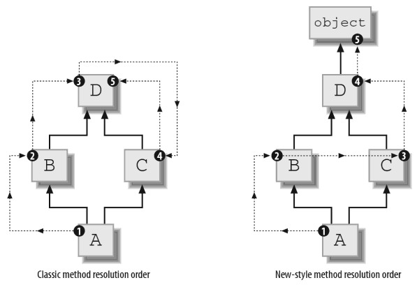
___mro___
Here is the code to prove that what we just discussed is true:
>>> class D:
... pass
...
...
>>> class B(D):
... pass
...
...
>>> class C(D):
... pass
...
...
>>> class A(B, C):
... pass
...
...
>>> D.__bases__
(<class 'object'>,) # D is a new-style class/type
>>> A.__bases__
(<class '__main__.B'>, <class '__main__.C'>)
>>> A.__mro__
(<class '__main__.A'>, # left-to-right then depth-first
<class '__main__.B'>,
<class '__main__.C'>,
<class '__main__.D'>,
<class 'object'>)
>>>
Now what is __mro__? Each new-style class/type has a special read-only
class attribute called __mro__. It is a tuple containing the
class/type MRO, in order. __mro__ only exists on a class/type but not
on instances thereof, and since it is read-only, it can not be
rebound/unbound.
Shadowing/Overriding Attributes
In Python we can shadow/override any type of attribute, whether it is
a callable or just a simple literal.
MRO is important when it comes to shadowing/overriding attributes
during inheritance. Examples and explanations are gives here and here.
Delegating Calls to Superclass/Supertype
Quite often we want to delegate calls to a callable (e.g. a method)
from a subclass/subtype to its superclass/supertype because the very
same callable might have been shadowed/overridden in the
subclass/subtype. Doing so is made easy using an unbound method:
>>> class Foo:
... def greet(self, *args, **kwargs):
... print("Hello {}!".format(args[0]))
...
...
...
>>> class Bar(Foo):
... def greet(self, *args, **kwargs):
... print("inside Bar.greet")
... Foo.greet(self, *args, **kwargs) # using an unbound method with explicit self
...
...
...
>>> baz = Bar()
>>> baz.greet("World")
inside Bar.greet
Hello World! # we delegated the call from Bar.greet to Foo.greet
>>> Bar.__bases__
(<class '__main__.Foo'>,)
>>> Bar.__mro__
(<class '__main__.Bar'>,
<class '__main__.Foo'>,
<class 'object'>)
>>>
With this example we used an unbound method in Bar in order to
delegate a method call to its superclass/supertype Foo. In fact, one
of the most common use cases for unbound methods is with delegating
calls to some other class/type, most likely a superclass/supertype.
For example, delegating from a subclass/subtype's __init__ to its
superclass/supertype's __init__ is common practice because otherwise
we would end up with this:
>>> class Foo:
... def __init__(self, *args, **kwargs):
... self.name = kwargs['name']
...
>>> class Bar(Foo):
... def __init__(self, *args, **kwargs):
... self.type = kwargs['type']
...
...
...
>>> Bar.__mro__
(<class '__main__.Bar'>,
<class '__main__.Foo'>,
<class 'object'>)
>>> fiz = Bar(type="cat", name="mister")
>>> fiz.__dict__
{'type': 'cat'} # poor cat, it does not even have a name
>>>
What happened? What is the problem? Well, the problem is that although
Bar subclasses Foo, obviously instances of Bar do not get created with
a name attribute but only with a type attribute. The reason for this
is simple, Foo.__init__ is not called when we instantiate fiz, which
is an instance of Bar.
Ideally, in nine out of ten cases, what we want is that when we
instantiate fiz, first Foo.__init__ is called and then Bar.__init__ is
called so that our poor cat does not end up without a name.
What we could do is to simply use our unbound method trick again and
rewrite Bar (Foo is unchanged):
>>> class Bar(Foo):
... def __init__(self, *args, **kwargs):
... Foo.__init__(self, *args, **kwargs)
... self.type = kwargs['type']
...
...
...
>>> fiz = Bar(type="cat", name="mister")
>>> fiz.__dict__
{'name': 'mister', 'type': 'cat'} # mister! :-]
>>>
super
Now, using unbound methods like this works but is not quite versatile
plus hardcoding class/type names certainly is unpythonic. super() to
the rescue! Let us adopt our example even further (Foo is unchanged):
>>> class Bar(Foo):
... def __init__(self, *args, **kwargs):
... super().__init__(*args, **kwargs) # no more hardcoding class/type names
... self.type = kwargs['type']
...
...
...
>>> foz = Bar(type="cat", name="mister")
>>> foz.__dict__
{'name': 'mister', 'type': 'cat'}
>>>
What happened? Well, super() returns a proxy object (the built-in type
<class 'super'>) that takes MRO into account and
delegates method calls to a superclass/supertype or sibling
class/type. This is incredibly useful for accessing inherited
callables (e.g. methods) that have been shadowed/overridden. The
search order is same as used for getattr() except that the class/type
where the initial call initiates from is skipped.
There are two typical use cases for super()
- In a class/type hierarchy with single inheritance,
super() can be
used to refer to superclasses/supertypes without naming them
explicitly, thus making the code more maintainable. This use of
super() in Python closely parallels the use of super() in other
programming languages.
- The second use case is to support multiple inheritance in a
dynamic execution environment. This use case is unique to Python
and is not found in statically typed languages or languages that
only support single inheritance. This makes it possible to
implement diamond-shaped inheritance chains where multiple
superclasses/supertypes implement the same method. Good design
dictates that those methods have the same signature in every case
(because the order of calls is determined at run time, because
that order adapts to changes in the class/type hierarchy, and
because that order can include sibling classes/types that are
unknown prior to run time).
Using super() is recommended
In general it is considered good practice of always doing calls to
superclasses/supertypes using super() even if we do not have to deal
with multiple inheritance and thus the possibilities of diamond-shaped
inheritance chains.
Using super() is fine for the same reason that the majority of
true/false evaluations should not be done explicitly but rather
implicitly i.e. let Python do the work because it is smarter/faster
anyway. What that means with regards to super() is that our code
becomes more versatile, more reusable and easier to maintain as
opposed to what it would be would we hardcode things.
Composition
This is basically about combining basic data types into more complex
ones — assembling features/functionality, very much like what mixins
can be used for. Composition creates objects often referred to as
having a has a relationship e.g. car has a gearbox — this is
different to what inheritance does.
Inheritance is the process of adding details to a basic data type in
order to create a more specific one i.e. inheritance creates is a kind
of relationships e.g. car is a kind of vehicle.
Whether to chose inheritance or composition depends on particular use
case at hand. Inheritance is a more commonly-understood idea. Asking a
typical developer about composition will most likely result in some
mumbling and deflection, whereas the same question about inheritance
will probably reveal a whole host of opinions and experience. That is
not to say that composition is some sort of dark art, but simply that
it is less commonly talked about and even less often used.
As more of a sidenote than anything else, inheritance can be speedier
in some compiled languages due to some compile-time optimizations vs.
the dynamic lookup that composition requires. Of course, in Java we
cannot escape the dynamic method lookup, and in Python it is all a
moot point.
In the end, both, inheritance and composition, cater to the same
problem domain (building complex data types from/with simpler ones)
but achieve such through different ways.
Composition creates objects often referred to as having a has a
relationship (car has a gearbox) whereas inheritance is the process of
adding detail to a general data type to create a more specific data
type i.e. create a is a kind of relationship e.g. car is a kind of
vehicle.
The basic messages is that, as with many things in life, there is not
better as both ways depend on the use case in hand and more often than
not, personal preference of the individual programmer or the team
writing some piece of code.
Example
Before talking about the consequences of inheritance vs composition,
some simple examples of both are needed. Here is a simplistic example
of object composition:
class UserDetails:
"""A class that compiles blabla."""
email = "[email protected]"
homepage = ""
class User:
"""A class used to store blabla."""
first_name = "Markus"
last_name = "Gattol"
details = UserDetails()
Obviously these are not very useful classes, but the essential point
is that we have created a namespace for each User object called
details, which contains the extra information about that particular
user.
An example of the same objects, modified to use inheritance might look
as follows:
class User:
"""A class in charge of blabla."""
first_name = "Markus"
last_name = "Gattol"
class UserDetails(User):
"""A class blabla."""
email = "[email protected]"
homepage = ""
Now we have a flat namespace, which contains all of the attributes
from both of the objects. In the case of any collisions, Python will
take the attribute from UserDetails.
Consequences
From a pure programming language complexity standpoint, object
composition is the simpler of the two methods. In fact, the word
object may not even apply here, as it is possible to achieve this type
of composition using C structures, which are clearly not objects in
the sense that we think of them today.
Another immediate thing to notice is that with composition, there is
no possibility of namespace clashes. There is no need to determine
which attribute should win, between the object and the composed
object, as each attribute remains readily available.
The composed object has no knowledge about its containing class, so it
can completely encapsulate its particular functionality. This also
means that it cannot make any assumptions about its containing class,
and the entire scheme can be considered less brittle. Change an
attribute or method on User? That is fine, since UserDetails does not
know or care about User at all — that would be totally different in
case of inheritance.
That being said, object inheritance is arguably more straightforward.
After all, an e-mail address is not a logical property of some
real-world object called UserDetails (it is a property of a user) thus
it makes more sense to make it an attribute on our virtual equivalent,
the User class.
Conclusion
Most people using both find object composition to be desirable. The
reasons seems to be that many projects get incredibly (and
unnecessarily) confusing due to complicated inheritance hierarchies.
However, there are some cases where inheritance simply makes more
sense logically and programmatically. These are typically the cases
where an object has been broken into so many subcomponents that it
does not make sense any more as an object itself.
The Django web-framework for example has an interesting way of dealing
with model inheritance. It uses composition behind the scenes, and
then flattens the namespace according to typical inheritance rules.
However, this is done in a way so that composition still exists under
the covers which still allows composition to be used if
needed/desired.
The answer is not going to be composition always or inheritance always
or even any combination of the two, always, or even something similar
but not quite the same such as traits. Each has its drawbacks and
advantages and those should be considered before choosing any
approach. More research needs to be done on the hybrid approaches, as
well, because things like what Django is doing will provide more
answers to more people than traditional approaches.
Comprehension
Roughly speaking, comprehension denotes mathematical notation used to
represent infinite mathematical constructs. Comprehensions, with
regards to programming languages, are most closely associated with
Haskell, but are available in other languages such as Python, Scheme
and Common Lisp as well.
One type of comprehension found in Python is list comprehension. List
comprehension is greedy evaluation i.e. it computes the entire result
all at once, as a list. Generator expressions on the other hand do
lazy evaluation i.e. they computes one value at a time, when needed,
as individual values. This is especially useful for long/big sequences
where the computed list is just an intermediate step and not the final
result. Below are some examples of the types of comprehensions found
in Python:
1 >>> [n * n for n in range(5)] # list comprehension, greedy evaluation
2 [0, 1, 4, 9, 16]
3 >>> {n * n for n in range(5)} # set comprehension
4 {0, 1, 4, 16, 9}
5 >>> {n: n * n for n in range(5)} # dictionary comprehension
6 {0: 0, 1: 1, 2: 4, 3: 9, 4: 16}
7 >>> mygenerator = (n * n for n in range(5)) # generator expression, lazy evaluation
8 >>> mygenerator.__next__()
9 0
10 >>> mygenerator.__next__()
11 1
12 >>> mygenerator.__next__()
13 4
14 >>> mygenerator.__next__()
15 9
16 >>> mygenerator.__next__()
17 16
18 >>> mygenerator.__next__()
19 Traceback (most recent call last):
20 File "<stdin>", line 1, in <module>
21 StopIteration
22 >>>
As we can see, the generator expression returns an iterator for lazy
evaluation (lines 8 to 17). Once the iterator is exhausted because
there is no more data available from the stream, the StopIteration
exception is raised.
List Comprehension
List comprehension is a way of creating lists from sequences e.g.
other lists. In general, list comprehensions work quite similar to for
loops.
Common applications are to make lists where each item in the list is
the result of some operations applied to each item of a sequence, or,
to create a subsequence of those items that satisfy a certain
condition.
>>> somecontainer = [number * number for number in range(10)]
>>> print(somecontainer)
[0, 1, 4, 9, 16, 25, 36, 49, 64, 81]
>>> sum(somecontainer)
285
>>> type(somecontainer)
<class 'list'>
>>> somecontainer = [number * number for number in range(10) if number % 2]
>>> print(somecontainer)
[1, 9, 25, 49, 81]
>>>
In case we are only interested in the sum i.e. we do not need the
intermediate list of squares, it is smarter to use a
generator expression expression as it lazily produces values, one at a
time.
- Rule of thumb:
- We use a list comprehension when a computed list is the desired
result.
- We use a generator expression when the computed list is just an
intermediate step. Note however that this often happens
automatically. For example, with
for item in somecontainer: pass
i.e. a for loop Python, looks at the sequence supplied after the in
keyword (e.g. the list somecontainer). If it is a standard
container such as a list, tuple, dictionary, set, user-defined
container, etc. then Python converts it into an iterator
automatically. If it is already an iterator (e.g. because we used
the generator expression (n*n for n in range(3)) instead of
somecontainer), it is uses by Python directly.
Set Comprehension
Python 3 introduces set comprehensions. Similar in form to list
comprehensions, set comprehensions generate Python sets instead of
lists:
>>> {char for char in "ABCDABCD"}
{'A', 'C', 'B', 'D'}
>>> myset = {char for char in "ABCDABCD" if char not in "AD"}
>>> print(myset)
{'C', 'B'}
>>> type(myset)
<class 'set'>
>>>
Dictionary Comprehension
Also with Python 3, we got another nifty type of comprehension, namely
dictionary comprehension. Dict comprehensions can be used to create
dictionaries from arbitrary key/value expressions:
>>> {key: value for key, value in enumerate("ABCD")}
{0: 'A', 1: 'B', 2: 'C', 3: 'D'}
>>> somecontainer = {key: value for key, value in enumerate("ABCD") if value not in "CB"}
>>> print(somecontainer)
{0: 'A', 3: 'D'}
>>> type(somecontainer)
<class 'dict'>
>>> {key: pow(2, key) for key in (1, 2, 4, 6)}
{1: 2, 2: 4, 4: 16, 6: 64}
>>>
Here is a trick with dictionary comprehensions that might be useful
someday — swapping the keys and values of a dictionary:
>>> somecontainer = {'a': 1, 'b': 3, 'c': "foo"}
>>> somecontainer.keys()
dict_keys(['a', 'c', 'b'])
>>> somecontainer.values()
dict_values([1, 'foo', 3])
>>> somecontainer = {value: key for key, value in somecontainer.items()}
>>> somecontainer.keys()
dict_keys([3, 1, 'foo'])
>>> somecontainer.values()
dict_values(['b', 'a', 'c'])
>>>
Of course, this only works if the values of the dictionary are
immutable e.g. like strings, numbers or tuples for example. If we try
this with a dictionary which contains lists (which we know are
mutable sequences), then this will fail because a dictionary can not
have mutable types as its keys:
>>> somecontainer = {'a': 1, 'b': 3, 'c': ["a", "foo"]}
>>> somecontainer.keys()
dict_keys(['a', 'c', 'b'])
>>> somecontainer.values()
dict_values([1, ['a', 'foo'], 3])
>>> somecontainer = {value: key for key, value in somecontainer.items()}
Traceback (most recent call last):
File "<stdin>", line 1, in <module>
File "<stdin>", line 1, in <dictcomp>
TypeError: unhashable type: 'list'
>>>
Iterator
In Python iterators are everywhere, underlying everything, always just
out of sight.
For example, comprehensions and generators are one way to create
iterators. Another example are for loops as they
automatically attempt to convert a supplied sequence into an iterator
which yields the sequence's items or iterable objects, one by one.
An iterator is an object representing a stream of data made from
iterable objects e.g. characters from a string (in Python 3 a string
is a sequence of unicode characters). Repeated calls to the iterator's
__next__() (or passing it to the built-in function next()) method
return successive objects from the stream:
>>> myiterator = iter("big dog")
>>> type(myiterator)
<class 'str_iterator'>
>>> next(myiterator)
'b'
>>> next(myiterator)
'i'
>>> next(myiterator)
'g'
>>> next(myiterator)
' '
>>> next(myiterator)
'd'
>>> next(myiterator)
'o'
>>> next(myiterator)
'g'
>>> next(myiterator)
Traceback (most recent call last):
File "<input>", line 1, in <module>
StopIteration
>>>
When there is no more data available from the stream, a StopIteration
exception is raised. At this point, the iterator object is exhausted
and any further calls to its next() method just raise StopIteration
again.
Iterators are required to have an __iter__() method that returns the
iterator object itself so every iterator is also iterable and may be
used in most places where other iterables are accepted.
One notable exception is code which attempts multiple iteration
passes. A container object (such as a list) produces a fresh new
iterator each time we pass it to the iter() function or use it in a
for loop. Attempting this with an iterator will just return the same
exhausted iterator object used in the previous iteration pass, making
it appear like an empty container.
Now that we know about __next__() and __iter__() it is also time to
mention __reversed__(). It takes an existing sequence and returns an
iterator that yields the items in the sequence in reverse order, from
last to first. Implementing __reversed__() is optional.
__prev__(), __current__()
Many people would like to have additional functionality with regards
to iterators e.g. __prev__() to get the previous item, __current__()
to get the current item again, __finished__() to test whether the
iterator is finished, and maybe even others, like __rewind__(),
__len__(), __position__(). Have a look at PEP 234 why we do not have
them (yet).
itertools
how to flatten a nested lists
>>> tmp
[[u'tom'], [u'tom', u'tim']]
>>> from itertools import chain
>>> list(chain(*tmp))
[u'tom', u'tom', u'tim']
Iterable
A container object capable of returning its items one at a time rather
than all at once.
Examples of iterable objects include sequence types such as list, str,
or tuple as well as non-sequence types like dict, file and objects of
any classes we define with an __iter__() or __getitem__() method.
Iterables in for loops
Iterables can be used in a for loop and in many other places where a
sequence is needed (zip(), map()...). When an iterable object is
passed as an argument to the built-in function iter(), it returns an
iterator for the object. This iterator is good for one pass over the
set of values.
When using iterable objects, it is usually not necessary to call
iter() or deal with iterators. The for statement does that
automatically for us, creating a temporary unnamed variable to hold
the iterator for the duration of the for loop.
all()
Is the iterable empty? If not, are all items of the iterable true?
How do we test for an empty iterable i.e. one that does not contain
any items? We could do this
>>> myiterable = list(range(1, 4))
>>> myiterable
[1, 2, 3]
>>> def all(iterable):
... for item in iterable:
... if not item:
... return False
... return True
...
...
>>> all(myiterable) # all items are true...
True
>>> all([]) #... or iterable is empty
True
>>>
or... we could be smarter and just use the built-in function all()
;-]
>>> all
<function all at 0x7ff2e1a09af0> # our own all()
>>> del all
>>> all
<built-in function all> # now we have the built-in again
>>> all(myiterable)
True
>>> all([])
True
>>>
Note that we need to use del() (yet another built-in function) in
order to unshadow the built-in all() from our own all() which we
created earlier.
As can be seen, all() returns True if all items of the iterable are
true in a boolean context or if the iterable is empty. It returns
False when the iterable contains an item that is false in a boolean
context:
>>> myiterable = list(range(4))
>>> myiterable
[0, 1, 2, 3] # 0 evaluates to false in a boolean context
>>> all(myiterable)
False
>>>
When we start combining things like for example generator expressions
and all(), then we end up with one-liners that really do a lot in just
one line of code:
>>> myiterable = range(1, 4)
>>> list(myiterable)
[1, 2, 3]
>>> all(number != 0 for number in myiterable) # true if all items of myiterable are non-zero
True
>>> myiterable = range(4)
>>> all(number != 0 for number in myiterable)
False
>>>
In this case we check against the integer 0 which means that we should
do an explicit check against it (e.g. != 0) rather than
relying on implicit checks which is what is usually recommended with
most true/false evaluation cases.
any()
Is the iterable empty? If not, does it have at least one item that
is true? While all() is useful, any() is used a lot more in practice
because it is semantically closer to what we need to do a lot...
checking if any item in the iterable is true or, checking if the
iterable is empty.
Remember that all() would return True for an empty iterable but also
for an iterable which contains items that are all true in a boolean
context. Therefore, if we wanted to check for an empty iterable we
cannot be sure whether or not all(iterable) returns True because the
iterable is really empty or, because it is not empty but rather every
of its items is true.
If any(iterable) would return False however then we can sure that we
are dealing with an empty iterable i.e. we would need no further
checks to find out whether it is really empty or if it contains
items which are all true in a boolean context.
In short: any(iterable) returns True if any item of the iterable is
true. If the iterable is empty, then any(iterable) returns False. As
for all(), we can write this function on our own so that it is
semantically equivalent to the built-in any():
>>> def any(iterable):
... for item in iterable:
... if item:
... return True
... return False
...
...
>>> myiterable = list(range(1))
>>> myiterable
[0] # 0 evaluates to false in a boolean context
>>> any(myiterable)
False
>>> any([])
False
>>> myiterable = list(range(2))
>>> myiterable
[0, 1]
>>> any(myiterable)
True
>>>
Now, let us unshadow (remove the binding of the name any from the
local/global namespace) the built-in function any() by using the del
statement and try again:
>>> any
<function any at 0x7ff2e1a176b0> # our own any()
>>> del any
>>> any
<built-in function any> # now we have the built-in again
>>> any(myiterable)
True
>>> myiterable = "" # an empty string is an empty iterable too
>>> any(myiterable)
False
>>>
When we start combining things like for example generator expressions
and any(), then we end up with one-liners that really do a lot in just
one line of code:
>>> myiterable = range(5)
>>> list(myiterable)
[0, 1, 2, 3, 4]
>>> any(number > 3 for number in myiterable) # true if any item of myiterable is > 3
True
>>> myiterable = range(4)
>>> any(number > 3 for number in myiterable)
False
>>>
Descriptor
As for everything else in Python, a descriptor is an object too. A
python object is said to be a descriptor if it implements the the
so-called descriptor protocol.
In other words: An object which defines any of the __get__(),
__set__() or __delete__() special methods is said to implement the
descriptor protocol. There are two types of descriptors:
- An object that defines both, a
__get__() and a __set__()
special method is a data descriptor.
- An object that only defines a
__get__() special method is a
non-data descriptor (they are typically used for methods but other
uses are possible as well).
To make a read-only data descriptor we can define both special
methods, __get__() and __set__() but then we make it so that when
__set__() is called, it raises an AttributeError exception. The reason
why we might do that instead of simply having a non-data descriptor
has to do with different shadowing/overriding semantics of the two. It
is also quite useful when we want a read-only property.
Because descriptors are a powerful, general purpose protocol,
understanding the descriptor protocol is key to understanding Python's
innards because so many things in Python are based on it e.g.
functions, methods, properties, class methods, static methods, and
references to superclasses/supertypes, etc. Descriptors are used
throughout Python itself to implement new style classes introduced in
version 2.2, they also simplify the underlying C-code and offer a
flexible set of new tools for everyday Python programs.
Descriptor Protocol
Any object with a __get__() special method, and optionally __set__()
and __delete__() special methods, accepting specific parameters is
said to follow the descriptor protocol.
Such an object qualifies as a descriptor and can be placed inside a
class/type's or instance's __dict__ dictionary (said to be the owner)
to do something when the attribute with the object's name is accessed
(referenced, set or deleted).
Creating a Descriptor
Let us now have a look at how to create a descriptor:
>>> class BazBar: # real code would have docstrings
... def __get__(self, instance, owner=None):
... print("calling __get__()")
...
... def __set__(self, instance, value):
... print("calling __set__()")
...
... def __delete__(self, instance):
... print("calling __delete__()")
...
...
...
>>>
The methods making up the descriptor protocol only apply when an
instance of the class/type containing such method appears in an
owner's class/type (see bar below) i.e. the descriptor must be in
either the owner's class/type __dict__ or in one of its
superclasses/supertypes __dict__.
- __get__(self, instance, owner)
-
Called to get (e.g. by referencing i.e.
objectname.attributename) the
attribute of the owner class/type (class attribute access) or an
instance of that class/type (instance attribute access).
-
owner is always the owner class/type, while instance is the instance
that the attribute was accessed through, or None when the attribute is
accessed through owner. This special method should return the
(possibly dynamically computed) attribute value or raise an
AttributeError exception.
- __set__(self, instance, value)
-
Called to set (e.g. by assignment
objectname.attributename =
5) the attribute on instance instance of the owner's class to
the (new) value value.
- __delete__(self, instance)
-
Called to delete (e.g.
del objectname.attributename) the attribute on
instance instance of the owner's class.
Using a Descriptor
What we defined with BazBar above is a class/type that can be
instantiated to create a descriptor object. Let us now look at how we
can attach this descriptor object to a class/type (the so-called owner
class/type) and put it to work:
1 >>> class FooBaz: # the owner class/type
2 ... bar = BazBar() # attribute bar is now a descriptor
3 ...
4 ...
5 >>> niznoz = FooBaz()
6 >>> dir(FooBaz)
7 ['__class__',
8 '__delattr__',
9 '__dict__',
10
11
12 [skipping a lot of lines...]
13
14
15 '__str__',
16 '__subclasshook__',
17 '__weakref__',
18 'bar']
19 >>> FooBaz.__dict__['bar']
20 <__main__.BazBar object at 0x32a0d50>
21 >>> FooBaz.bar
22 calling __get__()
23 >>> dir(niznoz)
24 ['__class__',
25 '__delattr__',
26 '__dict__',
27
28
29 [skipping a lot of lines...]
30
31
32 '__weakref__',
33 'bar'] # bar is an attribute on instance niznoz and not
34 >>> niznoz.__dict__
35 {} # a key in niznoz's __dict__
36 >>> niznoz.bar
37 calling __get__()
38 >>> niznoz.bar = "setting a value by assignment"
39 calling __set__()
40 >>> niznoz.__dict__
41 {}
42 >>> niznoz.__dict__['bar'] = "force-set a value" # a different bar; not our descriptor
43 >>> niznoz.__dict__
44 {'bar': 'force-set a value'}
45 >>> niznoz.bar # accessing descriptor bar via instance
46 calling __get__()
47 >>> del niznoz.bar
48 calling __delete__()
49 >>> FooBaz.bar # accessing descriptor bar via class/type
50 calling __get__()
51 >>> FooBaz.bar = "set/replace value for key bar"
52 >>> FooBaz.bar
53 'set/replace value for key bar' # descriptor replaced on owner's class/type but
54 >>> FooBaz.__dict__['bar']
55 'set/replace value for key bar'
56 >>> niznoz.bar # because bar is an instance variable it is
57 calling __get__() # not replaced on its instance
58 >>> fuzfiz = FooBaz()
59 >>> fuzfiz.bar # bar on fuzfiz still is the class variable
60 'set/replace value for key bar'
61 >>>
First thing to note is with line 2 where we instantiate our descriptor
class/type BazBar and thereby create a descriptor object. In the very
same line we are also binding the name bar to this descriptor object
which effectively means that from here on, every time the attribute
bar is accessed, either through its owner class/type FooBaz or one of
its instances (e.g. niznoz), our descriptor gets called (assuming its
not shadowed/overridden).
The circle is closed in line 5 where we instantiate the owner
class/type, thereby creating an object that has an attribute bar
which, under the hood, is managed using the descriptor as specified by
class/type BazBar.
Lines 6 to 37: If we now take a closer look at our owner class/type
FooBaz and its instance niznoz, we will see that while FooBaz's
__dict__ has a key bar, niznoz's __dict__ is empty. What that means
is that the name bar is a top-level attribute on niznoz bound to our
descriptor object rather than being a key inside its __dict__
dictionary — this fact can be exploited when we want to
shadow/override a non-data descriptor but it is also important with
regards how setting attributes on instances of owner classes work
which brings us right to the next fact.
As we can see from line 38, setting/updating a value for bar goes
through our descriptor. The __dict__ remains untouched. However, what
if we decided to directly insert into niznoz.__dict__? That works as
can be seen from lines 42 to 44. However, doing so does not touch our
descriptor at all (lines 44 to 46).
For the sake of completeness, lines 47 and 48 show how to delete
attribute bar or better said, what machinery is triggered by trying to
do so — whether or not bar gets deleted or not, when and how, all
depends on the implementation of __delete__() on our descriptor
class/type (BazBar in our example).
If we compare line 49 to e.g. line 45 then we can see how attribute
access can either happen trough the class or trough the instance. Note
however that when accessed from the owner class/type itself, only the
__get__() special method comes in the picture, setting or deleting the
attribute will actually replace or remove the descriptor as shown in
lines 51 to 55. Therefore, an important thing to realize is that when
we rebind the name bar on our owner class/type (FooBaz) then we
effectively replace our descriptor object with an ordinary attribute.
The consequence of doing so can be explained trough
class vs instance variables — the immediate results are shown in
lines 56 to 60.
One last important thing to note is that descriptors only work when
attached to classes/types (e.g. FooBaz in our example). Sticking a
descriptor in an object that is not a class/type gives us nothing.
Invoking Descriptors
A descriptor is an object attribute with binding behavior i.e. any
attribute on an object whose attribute access has been overridden by
methods in the descriptor protocol (__get__(), __set__(), and
__delete__()) binds attribute access to one of those three methods.
When an object's attribute is a descriptor, its special binding
behavior is triggered upon attribute access. For example, with an
instance a, using a.b is used to access (get, set or delete) attribute
b on object a — Python's look up chain starts with a.__dict__['b'],
then type(a).__dict__['b'], and then continues through the
superclasses/supertypes of type(a) excluding metaclasses (see MRO
(Method Resolution Order) for details) and returns its value.
However, if during attribute access it turns out that b is actually a
descriptor (maybe even a shadowing/overriding one from the instance's
class/type or one of its classes/types superclasses/supertypes), then
one of the respective descriptor methods on object b gets called
instead and whatever the result of that call might be gets returned to
the caller.
Anyhow, the important point to remember is that the starting point for
descriptor invocation is a binding such as objectname.attributename
(a.b in our current example). How the arguments are assembled depends
on a:
- Direct Call
-
The simplest and least common call is when our source code directly
invokes a descriptor method e.g.
b.__get__(a).
- Instance Binding
-
If binding to an object instance,
a.b is transformed to a call such as
for example type(a).__dict__['b'].__get__(a, type(a)).
- Class Binding
-
If binding to a class/type such as for example
FizFoo.b, then the call
is transformed into: FizFoo.__dict__['b'].__get__(None, FizFoo). Note
how we use None as first argument now. That is because we do not have
an instance, just the class/type itself.
- Super Binding
-
If
a is an instance of super, then the binding super(BazFiz, obj).m()
searches obj.__class__.__mro__ for the superclass/supertype FizFoo
immediately preceding BazFiz and then invokes the descriptor with the
call: FizFoo.__dict__['m'].__get__(obj, obj.__class__).
For instance bindings, the precedence of descriptor invocation depends
on the which descriptor methods are defined. A descriptor can define
any combination of __get__(), __set__() and __delete__()
special methods.
If it does not define __get__(), then accessing the attribute will
return the descriptor object itself unless there is a value in the
object's instance __dict__ dictionary. If the descriptor defines
__set__() and/or __delete__(), it is a so-called data descriptor. If
it defines neither, it is a so-called non-data descriptor.
Normally, data descriptors define both __get__() and __set__(), while
non-data descriptors have just the __get__() method. Data descriptors
with __set__() and __get__() defined always shadow/override a
redefinition in an instance dictionary. In contrast, non-data
descriptors can be overridden by instances.
Python methods (including static methods and class methods) are
implemented as non-data descriptors. Accordingly, instances can
redefine and shadow/override methods. This allows individual instances
to acquire behaviors that differ from other instances of the same
class. Properties on the other hand are data descriptors. Accordingly,
instances cannot override the behavior of a property.
Faith of Descriptors is with __getattribute__()
We already know that __getattribute__() is used to
customize attribute access. The main thing to know about it is that it
is called unconditionally. In addition to what is known about
__getattribute__() so far, it is also important to know that it also
determines how/if descriptors are called at all, and if so, which
methods in the descriptor protocol ( __get__(), __set__(), and
__delete__()) are called.
Extending on the example from above... The details of invocation
depend on whether obj is a class/type or an instance thereof. Either
way, descriptors only work for new style classes/types which were
introduced with Python 2.2 — we already know that a class/type is new
style if it is a subclass/subtype of object.
- instances
-
For instances, the machinery is in
object.__getattribute__() which
transforms a.b into type(a).__dict__['b'].__get__(a, type(a)).
-
The implementation works through a precedence chain that gives data
descriptors priority over instance variables, instance variables
priority over non-data descriptors, and assigns lowest priority to
__getattr__() if provided — see shadowing/overriding with regards to
attribute access for more details.
-
The full C implementation can be found in
PyObject_GenericGetAttr() in
../Objects/object.c.
- classes/types
-
For classes/types, the machinery is in
type.__getattribute__() which
transforms FizFoo.b into FizFoo.__dict__['b'].__get__(None, FizFoo).
- super
-
The object returned by super() also has a custom
__getattribute__()
method for invoking descriptors.
-
The call
super(BazFiz, obj).m() searches obj.__class__.__mro__ for the
superclass/supertype FizFoo immediately following BazFiz and then
returns FizFoo.__dict__['m'].__get__(obj, FizFoo). If not a
descriptor, m is returned unchanged.
-
If not in the dictionary,
m reverts to a search using
object.__getattribute__().
Summary
- Descriptors are invoked by the
__getattribute__() special method.
- Overriding
__getattribute__() prevents automatic calls to
descriptors from happening.
__getattribute__() is only available with new style classes/types.object.__getattribute__() and type.__getattribute__() make
different calls to __get__().- Data descriptors always shadow/override an entry in an instance's
__dict__ dictionary.
- Non-data descriptor may be shadowed/overridden by en entry in an an
instance's
__dict__ dictionary.
We now know that the mechanism for descriptor calls is embedded in the
__getattribute__() special methods for object, type, and super().
Classes/types inherit this machinery when they derive from object or
if they have a metaclass/metatype providing similar functionality.
Likewise, classes/types can turn off calls to descriptors by
shadowing/overriding __getattribute__().
Shadowing/Overriding
Overall attribute lookup/reference semantics not only depends on
inheritance and thus MRO (Method Resolution Order) but is also
determined by which type of descriptor is involved i.e. data
descriptors and non-data descriptors differ in how
shadowing/overriding them works with respect to entries in an
instance's dictionary and also how the overall faith of a descriptor
is determined.
- If an instance's dictionary has an entry with the same name as a
data descriptor, the data descriptor takes precedence i.e. it
shadows/overrides the binding for the same name in the instance's
dictionary.
- If an instance's dictionary has an entry with the same name as a
non-data descriptor, the dictionary entry takes precedence i.e.
non-data descriptors can be shadowed/overridden on instances.
Python methods (including static methods and class methods) are
implemented as non-data descriptors. Accordingly, instances can rebind
and thereby shadow/override methods. This allows individual instances
to acquire behaviors that differ from other instances of the same
class/type. The property() built-in function is implemented as a data
descriptor i.e. instances cannot shadow/override the behavior of a
property.
Data Descriptor
Any object that has both, a __get__(), a __set__() and possibly a
__delete__() special method defined, is a data descriptor. As for
non-data descriptors, data descriptors have distinct semantics with
regards to shadowing/overriding and at which point in the
precedence chain they are called.
Property
A property is a data descriptor, created using the property()
built-in function. Properties are used for accessing attributes where
we would otherwise have used getter, setter and deleter methods. In
other words, properties are a way to wrap method calls for getting and
setting attributes as standard attribute access when the computation
is lightweight.
Benefits
Readability is increased by eliminating explicit get() and set()
method calls for attribute access. Properties allow possible
calculations to be lazy. They are also considered the pythonic way to
maintain an interface of a class/type because by using them we can
maintain a stable API (Application Programming Interface) and still
alter its implementation if need be.
In terms of performance, its possible to bypass properties using
trivial accessor methods which directly access attributes. This also
allows accessor methods to be added in the future without breaking the
interface. However, one should keep in mind that such practices of
bypassing a property are generally frowned upon because they harm
readability and simplicity of our source code.
Downsides
Looking at source code, we will see that a property function is
textually specified after its getter and setter methods, requiring one
to notice they are used for a property further down. That of course is
not true when using the @property decorator which goes before the
getter method (named after the attribute itself) and is used to
implement read-only properties.
If we are not careful/diligent we might manage to hide side-effects
using properties, much like mistakes made with regards to operator
overloading. For example, inheritance with properties can be
non-obvious if the property itself is not shadowed/overridden. In this
case we must make sure that getter methods are called indirectly to
ensure methods shadowed/overridden in subclasses/subtypes are called
by the property.
Example
It is recommended to use properties to get or set attributes where we
would normally have used getter and setter methods. Read-only
properties should be created using the @property decorator.
1 >>> class Foo: # real code would have docstrings
2 ... def get_bar(self):
3 ... return self.__bar
4 ...
5 ... def set_bar(self, value):
6 ... self.__bar = value
7 ...
8 ... def del_bar(self):
9 ... del self.__bar
10 ...
11 ... bar = property(get_bar, set_bar, del_bar, "docstring... lorem ipsum")
12 ...
13 ...
14 ...
15 >>> Foo.bar
16 <property object at 0x1e2f260>
17 >>> Foo.__dict__
18 <dict_proxy object at 0x1e21130>
19 >>> Foo.__dict__['bar']
20 <property object at 0x1e2f260>
21 >>> type(Foo.__dict__['bar'])
22 <class 'property'>
23 >>> fiz = Foo()
24 >>> fiz.bar
25 Traceback (most recent call last):
26 File "<input>", line 1, in <module>
27 File "<input>", line 3, in get_bar
28 AttributeError: 'Foo' object has no attribute '_Foo__bar'
29 >>> fiz.bar = 3
30 >>> fiz.bar
31 3
32 >>> del fiz.bar
33 >>> fiz.bar
34 Traceback (most recent call last):
35 File "<input>", line 1, in <module>
36 File "<input>", line 3, in get_bar
37 AttributeError: 'Foo' object has no attribute '_Foo__bar'
38 >>> fiz.bar = range(4)
39 >>> fiz.bar
40 range(0, 4)
41 >>> type(fiz.bar)
42 <class 'range'>
43 >>> list(fiz.bar)
44 [0, 1, 2, 3]
45 >>> Foo.bar.__doc__
46 'docstring... lorem ipsum'
47 >>>
A property provides an easy way to call functions whenever an
attribute is accessed (referenced, set or deleted) on the instance.
When the attribute is referenced from the class/type, the getter
method is not called but the property object itself (lines 15 to 22)
is returned. A docstring can also be provided as can be seen in lines
lines 11 as well as 45 and 46 respectively.
One might have noticed that we used a particular notation (lines 3, 6
and 9) for naming our attribute bar on the instance —
__bar is a
name prefixed with two leading underscores. This invokes name mangling
inside class Foo i.e. __baz becomes _Foo__baz. The rationale is that
by doing so we avoid name clashes with subclasses of Foo as the class
name gets encoded into the attribute name.
A final word about inheritance with regards to properties: subclassing
a class/type containing a property (e.g. Baz) and redefining the
getter or setter functions is not going to change the property. The
property object is holding on to the functions provided at the time it
was instantiated i.e. when triggered by an attribute access it will
not do some fancy lookup trough some inheritance chain in order to
find some possible currently shadowed/overridden function on some
superclass/supertype of its class/type.
Read-only/Non-deletable Properties
We already know that by default a property is always a
data-descriptor. However, as outlined in the beginning, in order to
make a read-only data descriptor the only thing we need to do is to
not defining all its special methods:
>>> class Baz:
... def get_it(self):
... pass
...
... def set_it(self, value):
... pass
...
... def del_it(self):
... pass
...
... full = property(get_it, set_it, del_it, "I can be referenced, set, and deleted.")
... nodelete = property(get_it, set_it, "I can be referenced, set, but not deleted.")
... readonly = property(get_it, "I can be referenced but not set or deleted.")
...
...
>>> foofiz = Baz()
>>> del foofiz.full
>>> del foofiz.nodelete
Traceback (most recent call last):
File "<input>", line 1, in <module>
TypeError: 'str' object is not callable
>>> foofiz.readonly = 4
Traceback (most recent call last):
File "<input>", line 1, in <module>
TypeError: 'str' object is not callable
>>> foofiz.full = 4
>>>
Nothing to say here as the example is self-explanatory...
@property
Now that we know how to create a read-only property why not go further
and use the pythonic way to do so. Doing read-only properties the
pythonic way means using a decorator. Meet @property everyone:
>>> class Maus: # real code would have docstrings
... def __init__(self):
... self._enemy = "Katze"
...
... @property
... def enemy(self):
... """Return Maus's worst enemy.""" # automatically becomes docstring
... return self._enemy
...
...
...
>>> baz = Maus()
>>> baz.enemy
'Katze'
>>> Maus.enemy.__doc__
"Return Maus's worst enemy."
>>>
This turns the enemy() method into a getter for a read-only attribute
with the same name.
More Decorators
A property object has getter, setter, and deleter methods usable as
decorators that create a copy of the property with the corresponding
accessor function set to the decorated function. This is best
explained with an example:
1 >>> class Bar:
2 ... def __init__(self):
3 ... self.__foo = None
4 ...
5 ... @property
6 ... def foo(self):
7 ... """I am the 'foo' attribute."""
8 ... return self.__foo
9 ...
10 ... @foo.setter
11 ... def foo(self, value):
12 ... self.__foo = value
13 ...
14 ... @foo.deleter
15 ... def foo(self):
16 ... del self.__foo
17 ...
18 ...
19 ...
20 >>> Bar.foo.__doc__
21 "I am the 'foo' attribute."
22 >>> Bar.foo.fget
23 <function foo at 0x1ea2ea8>
24 >>> Bar.foo.fset
25 <function foo at 0x1ea2d98>
26 >>> Bar.foo.fdel
27 <function foo at 0x1ead050>
28 >>> Bar.foo.getter
29 <built-in method getter of property object at 0x1eaa158>
30 >>> Bar.foo.setter
31 <built-in method setter of property object at 0x1eaa158>
32 >>> Bar.foo.deleter
33 <built-in method deleter of property object at 0x1eaa158>
34 >>> baz = Bar()
35 >>> baz.__dict__
36 {'_Bar__foo': None}
37 >>> baz.foo is None
38 True
39 >>> baz.foo = 5
40 >>> baz.__dict__
41 {'_Bar__foo': 5}
42 >>> del baz.foo
43 >>> baz.__dict__
44 {}
45 >>> baz.foo
46 Traceback (most recent call last):
47 File "<input>", line 1, in <module>
48 File "<input>", line 8, in foo
49 AttributeError: 'Bar' object has no attribute '_Bar__foo'
50 >>> Bar.foo.fget(baz)
51 >>> Bar.foo.fset(baz, 8)
52 >>> Bar.foo.fget(baz)
53 8
54 >>> baz.__dict__
55 {'_Bar__foo': 8}
56 >>>
The returned property object has the attributes fget, fset, and fdel
corresponding to the constructor arguments (lines 22 to 27 and 50 to
53).
The main thing to remember from this example is that we can see that
each property object has its built-in getter, setter and deleter
methods (lines 28 to 33) which we can use as decorators when prefixed
with the attribute name. This is the most concise way to work with
properties because we do not have to use an explicit property()
method. However, explicitly using foo = property(... )
would be more pythonic and is therefore favorable over this version.
We also decided again to prefix the attribute name (foo) with
two leading underscores in order to avoid name clashes with subclasses
of Bar.
Non-Data Descriptor
An object that only defines a __get__() special method is a non-data
descriptor. All Python methods (including static methods and
class methods) are implemented as non-data descriptors, which return
bound or unbound methods depending whether they are invoked from a
class/type or instance thereof.
As for data descriptors, non-data descriptors have distinct semantics
with regards to shadowing/overriding and at which point in the
precedence chain they are called.
Data Structures
In Python we have two groups of data structures —
literals and
containers, each of which have several subsets identified by certain
constraints and/or capabilities.
WRITEME
Data Structures - Literals
WRITEME
None
None became a keyword in Python 3, it is immutable and a frequently
used built-in constant used to signify the absence of a value,
basically being a placeholder, a so-called null value.
Equality and Subclassing
Generally speaking, we need to be careful when using None in a
boolean context as testing for equality (==) between None
and anything other than None will always return False:
>>> None == False
False
>>> None == True
False
>>> None == 0
False
>>> None == []
False
>>> None == None # only time the equality check returns True
True
>>>
None is the only null value in Python. It has its own datatype
(NoneType) and we can assign None to any variable, but we cannot
create other NoneType objects. All variables whose value is None are
equal to each other:
>>> type(None)
<class 'NoneType'>
>>> x = y = None
>>> x == None
True
>>> y == None
True
>>> x == y
True
>>> class MyNoneType(None):
... pass
...
...
Traceback (most recent call last):
File "<input>", line 1, in <module>
TypeError: cannot create 'NoneType' instances
>>>
None is a Singleton
None is a singleton i.e. there only ever exists one None at a time:
>>> None is None # identity check
True
>>> id(None) == id(None) # equality check of None's id
True
>>> id(None)
8794272
>>>
is None vs == None
Which one is better/correct? is checks to see if two objects are
actually one and the same object whereas == checks if
they are equal.
The short answer is that we should always use is None or is not None
(testing for identity/non-identity) rather than == None
or != None (testing for equality/inequality).
The long answer is that because there is the fact that
None is a singleton and that there is the general notion of
equality vs identity, checking some value against None using is is the
right thing to do but checking some value against None using
== is just plain wrong because it is ambiguous.
... is not None is preferred:
The is not operator is preferred over negating the result of is for
stylistic reasons: foo is not None reads just like everyday English,
but foo not x is None requires understanding of operator precedence
and is not very intuitive. Also, there is no performance difference
between the two as both produce the same bytecode:
>>> import dis
>>> def foo(bar):
... return bar is not None # this version is preferred
...
...
>>> dis.dis(foo)
2 0 LOAD_FAST 0 (bar)
3 LOAD_CONST 0 (None)
6 COMPARE_OP 9 (is not)
9 RETURN_VALUE
>>> def foo(bar):
... return not bar is None
...
...
>>> dis.dis(foo)
2 0 LOAD_FAST 0 (bar)
3 LOAD_CONST 0 (None)
6 COMPARE_OP 9 (is not)
9 RETURN_VALUE
>>>
Functions
An important thing to know is that None is returned from functions in
case they do not explicitly return anything. Another place where None
is used a lot is as a default parameter:
None as Default Parameter Value
Go here for more information.
Miscellaneous
Assignments to None raise a SyntaxError exception. The type of None is
NoneType. This type has a single value, None. There is a single object
with this value which is accessed through the built-in name None.
Ellipsis
The Ellipsis object is used to slice higher-dimensional data
structures. Its meaning is: Right here (location in multi-dimensional
slice e.g. array) insert as many full slices (:) as necessary in order
to extend the multi-dimensional slice to all available dimensions.
>>>...
Ellipsis
>>> Ellipsis
Ellipsis
>>> type(...)
<class 'ellipsis'>
>>> type(Ellipsis)
<class 'ellipsis'>
>>>
As we can see, ... is just syntactic sugar for Ellipsis. Both specify
the ellipsis object.
>>> Ellipsis is...
True
>>> ban =...
>>> bis =...
>>> boo = Ellipsis
>>> ban is boo
True
>>> ban is boo is bis
True
>>>
Ellipsis is a singleton i.e. there only ever exists one ellipsis
object at all times.
Practical Implications
So what are the practical implications with regards to the ellipsis
object? Well, there are none except for when we use the NumPy
extension. Or in other words, as long as we ever only deal with
one-dimensional slices (e.g. ordinary sequence types such as lists)
then we will not encounter ellipsis.
Ellipsis is used mainly by NumPy, which adds a multidimensional array
type (numpy.ndarray). Since there is more than one dimensions, slicing
becomes more complex than just specifying a start and stop index — it
is necessary to be able to slice in multiple dimensions as well. For
example given a 4x3 array, the 2x2 top left area would be specified by
the slice [:2, :2]:
>>> from numpy import arange
>>> arange(12).reshape(4, 3)
array([[ 0, 1, 2],
[ 3, 4, 5],
[ 6, 7, 8],
[ 9, 10, 11]])
>>> arange(12).reshape(4, 3)[:2, :2]
array([[0, 1],
[3, 4]])
>>> type(arange(12).reshape(4, 3)[:2, :2])
<type 'numpy.ndarray'> # multidimensional array type
>>>
The ellipsis object is used as a placeholder for the array dimensions
not specified. We can think of it as indicating the full slice [:] for
dimensions not specified e.g. for a three dimensional array
somefoo[..., 0] is the same as somefoo[:, :, 0]. Let us have a look at
our example which has two dimensions (4x3) and how we can use the
notation (... or Ellipsis respectively) for the ellipsis object:
>>> arange(12).reshape(4, 3)[..., :2] # placeholder specifying notation
array([[ 0, 1],
[ 3, 4],
[ 6, 7],
[ 9, 10]])
>>> arange(12).reshape(4, 3)[:4, :2]
array([[ 0, 1],
[ 3, 4],
[ 6, 7],
[ 9, 10]])
>>>
That is pretty much it with regards to the ellipsis object. Those who
want to know more should just install NumPy and start toying around.
NotImplemented
Numbers
Integral
Integer
Boolean
- http://docs.python.org/dev/library/stdtypes.html#truth-value-testing
- http://docs.python.org/dev/library/stdtypes.html#boolean-operations-and-or-not
- False:
NoneFalse- zero of any numeric type, for example,
0, 0.0, 0j
- any empty sequence, for example,
'', (), []
- any empty mapping, for example,
{}
- instances of user-defined classes, if the class defines a
__bool__() or __len__() method, when that method returns the
integer zero or bool value False.
- True: everything not mentioned under False e.g.
True
Operations and built-in functions that have a Boolean result always
return 0 or False for false and 1 or True for true, unless otherwise
stated. (Important exception: the Boolean operations or and and always
return one of their operands.)
Real/Float
Binary Floating Point
Decimal Floating Point
Because I wanted a Money data type...
— Facundo Batista
Decimal vs Binary Floating Point
- decimal floating point numbers have higher precision but require
more CPU cycles i.e. they are slower to compute and work with than
binary floating point
- from
/usr/lib/python3.2/numbers.py
- Decimal has all of the methods specified by the Real
abstract superclass/supertype, but it should not be registered as
a Real because decimals do not interoperate with binary floats
i.e. Decimal('3.14') + 2.71828 is undefined. But, abstract reals
are expected to interoperate i.e. R1 + R2 should be expected to
work if R1 and R2 are both reals.
- Decimals are not interoperable with floats and vice versa i.e. we
should not subclass Decimal from
numbers.Real and also not
register it as such
WRITEME
Complex
Data Structures - Containers
Some objects contain references to other objects. These are called
containers. The most prominent examples of containers are tuples,
lists and dictionaries. This section will look at those afore
mentioned types as well as others, not so prominent container types.
WRITEME
Sequences
Immutable Sequences
Strings
String
>>> import string
>>> string.ascii_letters
'abcdefghijklmnopqrstuvwxyzABCDEFGHIJKLMNOPQRSTUVWXYZ'
>>> string.punctuation
'!"#$%&\'()*+,-./:;<=>?@[\\]^_`{|}~'
>>> string.whitespace
'\t\n\x0b\x0c\r '
>>>
UserString
String Formatting
Tuple
Named Tuple
WRITEME
Named Tuple vs Foo
Before we start let us look at some questions often raised, namely
what is difference amongst named tuples and a punch of other data
structures in Python:
- Tuple vs List
-
Even if semantically speaking tuples and lists are not very different,
their use cases are.
- Named Tuple vs Tuple
-
Named tuples are tuples, they have the same semantics and can be used
to solve the same problems e.g. we can use named tuples as well as
tuples in for loops. It is best to think of named tuples as an
additional layer on top of ordinary tuples which adds support for
name-based access (setting, referencing, deleting items) in addition
to index-based access on ordinary tuples.
-
There are also a bunch of additional functions and features shipped
with this layer, but in a nutshell that is it: named tuples are tuples
which allow us to access items not just by index but also by name.
-
So, that is how tuples and named tuples differ, both are apples really
but one type just tastes a bit sweeter and gives us more drive in case
we need it...
- Named Tuple vs Dictionary
-
Tuples and named tuples are immutable sequences. Dictionaries are not
even sequence types but container types. So that is not apples and
apples but apples and oranges...
-
However, the main reason this questions is justified nonetheless is
because to many named tuples feel/look like dictionaries at first
glance even though most people know that they semantically totally
different, very much like apples and oranges totally different...
-
The real difference between the two quickly becomes apparent when we
look at the problem domains and use cases to which they are applied.
For example, if we use a dictionary in a for loop then we have to call
e.g.
somedict.values() rather than just supply the named tuple or
tuple for that matter. One of the main use cases for named tuples is
with having a pristine record type in Python for the first time,
something many people wanted for a long time before named tuples
arrived — even though we could always do a custom class/type and
create our own record types.
-
That is how different they are... apples and oranges, really!
Examples
>>> import datetime
>>> foo = datetime.datetime.utcnow()
>>> bar = foo.timetuple()
>>> bar
time.struct_time(tm_year=2011, tm_mon=2, tm_mday=21, tm_hour=16, tm_min=47, tm_sec=45, tm_wday=0, tm_yday=52, tm_isdst=-1)
>>> type(bar)
<class 'time.struct_time'>
>>> print(bar[0])
2011
>>> print(bar.tm_year)
2011
>>>
Byte
Range
Mutable Sequences
Lists
UserList
Deque
Byte Array
Miscellaneous
Sequence Comparison
Sequences can be compared in case their current objects under
comparison are of the same type:
>>> [1, 3] > [1, 4]
False
>>> [1, 3] > [1, 2]
True
>>> [1, 3] > [1, 2, 3]
True
>>> [1.11, 3] > [1, 2, 3]
True
>>> [1.11, 3] > [1, 2.447, 3]
True
>>> [1, 3] > [1, 2.447, "astring"] # decision can be made on [1]
True
>>> [1, 3] > [1, "astring"] # [1] has different types thus fails
Traceback (most recent call last):
File "<input>", line 1, in <module>
TypeError: unorderable types: int() > str()
>>>
The comparison uses lexicographical ordering i.e. first the first two
items ([0]) are compared, and if they differ this determines the
outcome of the comparison, we are done. On the other hand, if they are
equal, the next two items ([1]) are compared, and so on, until
either sequence is exhausted. If two items to be compared are
themselves sequences of the same type, the lexicographical comparison
is carried out recursively.
If all items of two sequences compare equal, the sequences are
considered equal. If one sequence is an initial sub-sequence of the
other, the shorter sequence is the smaller (lesser) one.
Lexicographical ordering for strings in Python uses the ASCII ordering
for individual characters.
>>> ord("a")
97
>>> chr("97") # the reverse
'a'
>>> ord("b")
98
>>> "a" > "b"
False
>>> "a" < "b"
True
>>> "ab" < "a"
False
>>> import pymongo
>>> pymongo.version
'1.9+'
>>> ord(".")
46
>>> ord("+")
43
>>> pymongo.version > "1.8"
True
>>> pymongo.version[2] > "1.8"[2]
True
>>> pymongo.version[2]
'9'
>>> "1.8"[2]
'8'
>>> pymongo.version[:2] == "1.8"[:2] # up to [2] they are equal
True
>>> pymongo.version[:2]
'1.'
>>> "1.8"[:2]
'1.'
>>>
Comparing objects of different types with < or > is legal provided
that the objects have appropriate comparison methods. For example,
mixed numeric types are compared according to their numeric value:
>>> 0 < 0.0
False
>>> 0 == 0.0
True
>>> 0.8 >= 0.8
True
>>> 0.83 > 0.8
True
>>> 0.8 > 0.8
False
>>>
Otherwise, rather than providing an arbitrary ordering, the
interpreter will raise a TypeError exception:
>>> "some string" > [1, 5]
Traceback (most recent call last):
File "<input>", line 1, in <module>
TypeError: unorderable types: str() > list()
>>>
Sets
- These represent unordered, finite sets of unique, immutable
objects. As such, they cannot be indexed by any subscript.
WRITEME
Set
Frozenset
Mappings
Dictionaries
- keys need be immutable types
Dictionary
UserDict
DefaultDict
OrderedDict
ChainMap
Counter
securedict
View
The objects returned from dict.keys(), dict.values(), and dict.items()
are called dictionary views. They provide a dynamic/lazy view on the
dictionary's entries which means that when the dictionary changes, the
view automatically reflects those changes (lines 5 to 7; keys being
the current view). To force the dictionary view to become a list
list(dictview) can be used (lines 8 and 9; and subsection further
down):
1 >>> somecontainer = {'one': 1, 'foo': 5}
2 >>> keys = somecontainer.keys()
3 >>> keys
4 dict_keys(['foo', 'one'])
5 >>> somecontainer['bar'] = 2
6 >>> keys
7 dict_keys(['foo', 'bar', 'one'])
8 >>> list(keys)
9 ['foo', 'bar', 'one']
Python 2 vs Python 3
In Python 2 views have to be explicitly created (e.g. by using
viewkeys(), introduced in Python 2.7) i.e. Python 2 returns lists
where Python 3 returns views:
| Python 2 |
Python 3 |
dict.keys() |
list(dict.keys()) |
dict.values() |
list(dict.values()) |
dict.items() |
list(dict.items()) |
dict.iterkeys() |
iter(dict.keys()) |
[i for i in dict.iterkeys()] |
[i for i in dict.keys()] |
This is how the syntax changes from Python 2 to Python 3 for doing
semantically the same thing. As mentioned further down, the point is
that we should now use dict.keys() and friends because they are more
efficient and concise.
View vs Iterator
Note that views are semantically somewhat hovering in between lists
and iterators — view objects returned by dict.keys() in Python 3 are
iterable (an iterator can be made from them). When we say
for key in dict.keys():
pass
Python will create an iterator for us. In Python 3, dict.keys()
returns a dict_keys object (lines 4 and 7) but if we use it in a for
loop then an iterator is created implicitly. In other words: the
difference between
for key in dict.keys():
pass
and
for key in iter(dict.keys()):
pass
is one of implicit vs explicit creation of the iterator. Whilst both,
views and iterators are lazy evaluation, we need to remember that if
we create an explicit iterator (line 14) then it can only be used once
(lines 17 to 20) whereas a view can be reused as often as required:
10 >>> "foo" in keys
11 True
12 >>> "bar" in keys
13 True
14 >>> myiterator = iter(somecontainer.keys())
15 >>> "foo" in myiterator
16 True
17 >>> "bar" in myiterator
18 True
19 >>> "bar" in myiterator
20 False
21 >>> "bar" in keys
22 True
23 >>> "bar" in keys
24 True
Also, notice that if we create an explicit iterator (line 25) and then
modify the dictionary after creating the iterator (line 26), then the
iterator is invalidated
25 >>> anotheriterator = iter(somecontainer.keys())
26 >>> somecontainer['cheese'] = 7
27 >>> for key in anotheriterator:
28 ... print(key)
29 ...
30 Traceback (most recent call last):
31 File "<stdin>", line 1, in <module>
32 RuntimeError: dictionary changed size during iteration
something that is not true if we use a view
33 >>> for key in keys:
34 ... print(key)
35 ...
36 cheese
37 foo
38 bar
39 one
40 >>> type(keys)
41 <class 'dict_keys'>
42 >>> type(somecontainer)
43 <class 'dict'>
44 >>> type(anotheriterator)
45 <class 'dict_keyiterator'>
46 >>> keys
47 dict_keys(['cheese', 'foo', 'bar', 'one'])
48 >>>
As we can see, we are still using the same view (keys) as initially
created in line 2... when the dictionary changes, the view
automatically reflects those changes...
Quality Assurance
High-quality products that are simple to use, with short time to
market cycles and top-notch customer support... Get this right and
consider yourself a winner, do not and you go out of business quickly.
Quality assurance for a software product encompasses the whole set of
requirements definition, software design, coding conventions,
software configuration management, peer review, issue tracking, change
management, testing, debugging, release management, and product
integration — all this without over-engineering things, with building
and keeping momentum as a team and with keeping the fun-factor and
excitement for developers alive...

All that might sound awfully complicated but in reality it is not that
hard to accomplish because there is often a lot of overlap among those
areas and not everything is needed for every project.
- Assuming we use GIT for software configuration management, it
makes sense to use Github. This also solves the issue tracking
problem since we can use Github's issue tracking system. If for
some reason that is not an option, it is easy to
setup our own GIT hosting on one of our own machines. While GIT is
a good tool for doing SCM, it is not so much the tool that matters
i.e. we could as well use any other SCM tool (hg, bzr...). What
matters is the process and having everybody pushing in the same
direction...
- We further assume that developers are experienced, that they are
team players who put the common goal before their individual egos,
and that they adhere to a certain coding style, that peer review
is a given, and that the development model in use is TDD
(Test-driven Development). Practice shows that, more often than
not, a small team of excellent developers capable of teamplay will
achieve better results faster than a big team of non-excellent
developers incapable of teamplay.
- What is left to do is to set up and maintain a system/process that
allows for continuous integration/deployment so that we end up
with a situation where we have a continuous flow of new features
which get tested and deployed to production automatically.
- We want to have software metrics built into our software so that
we gather information on business values that matter to our users
and therefore our business. We can then monitor the metrics for
those business values, much like the well-established monitoring
of basic things like diskspace, network, load...
This section assumes that we managed to accomplished #1 and #2
already. In order to satisfy #3 we need to have checks, tests and a
system that can run those checks and tests automatically every time
new code is checked into the repository.
At this point (December 2011) it seems that #4 is only done by a
minority of software projects. The notion of building metrics for
business values into software as we write it is quite new and not in
widespread use yet. This is going to change because people already
start realizing the importance of having accurate information on
business values of their software when it is running in production.
The remainder of this section will focus on #3 and #4 but will
initially also have a quick look at parts of #2 e.g. peer review and
TDD. Our goal is to end up with a set of processes and systems which
allows us to do quality assurance for the systems we build.
Design Documents
Design documents help us in managing complexity and synchronizing
people from different backgrounds. Projects above a certain size and
scale are not manageable without having design documents. That being
said, even for small projects it is worth doing them because they help
us catch flaws in mental models early in the process, thus saving a
lot of time and hassle down the road.
Depending on the design document, some of them are living documents as
they are constantly being amended to reflect a change of state and/or
goals set. As for most things with quality assurance, the key to
design documents is to not create to much of a burden — only if
things are simple and show benefits rather quickly will people do
them...
The danger with design documents is that the whole process can easily
become to theoretical/complex which will then lead to two different
worlds existing in parallel — the one on paper and what happens on
the ground. To avoid this we should keep things simple — simplicity
is good, simplicity scales, simplicity shortens product cycles,
simplicity helps reduce time to market and last but not least,
simplicity makes for better quality...
Another thing that is very important but forgotten a lot is that we
should design for testability. Again, that is easy if we keep things
simple but unfeasible if we over-complicate things by over-engineering
them and/or add features just for the sake of features even if nobody
needs them.
Usually when we design systems then we have to think about hardware
and software, about users, about the business model, and the
business values which are going to matter. Our design has to account
for scalability as we usually start rather small.
One thing that is usually true is that rather than having a small
number of big and complex systems, it is preferable to have a big
number of small and simple systems — reasons why we would want this
are maintainability, usability, flexibility and redundancy. Cost (per
user/task, TCO...) and reduced vendor lock-in are two more reasons.
Among others, those reasons are key in creating a
high-quality product. Quality assurance and success really starts with
design and I can therefore not stress its importance often enough.
User Requirements Document
A URD is a document written from the point of view of a
(non-technical) user. It should be short (three pages or less). It
does not contain tech-jargon but words and descriptions non-technical
people would use. This is because often users are not able to
communicate the entirety of their needs and wants, and the information
they provide may also be incomplete, inaccurate and self-conflicting.
The responsibility of completely understanding what users want then
falls to us, the providers of the product.
Once the required information is completely gathered it is documented
in the URD, which is meant to spell out exactly what the system must
do and becomes part of the contractual agreement — or just the
internal URD in case we are planning for a system that users use
online.
A user cannot demand features not in the URD without renegotiating and
a developer cannot claim the product is ready if it does not meet an
item of the URD. The URD can be used as a guide to planning cost,
timetables, milestones, testing, etc.
The explicit nature of the URD allows users to show it to various
stakeholders to make sure all necessary features are described.
Formulating a URD requires negotiation to determine what is
technically and economically feasible.
Writing a URD is part science and part art as it requires both,
technical skills and interpersonal skills. People able to write such
documents are scarce — non-technicians tend to produce a lot of
blablabla, thereby failing to express and pin-down the essence that
matters mid to long-term. Most technicians on the other hand would
deliver a technical document that lacks creativity and does not
reflect the needs and ideas of the majority of users.
Market Requirements Document
This one is the seconds non-technical document after the URD that
people tend to write. However, whether or not we would do a MRD
depends on whether or not there is a commercial angle at play
(military and science projects often do not have a commercial angle to
them).
A MRD is a document that expresses the users wants and needs for a
product or service. It should explain what (new) product is being
discussed (referencing the URD is usually fine), the targeted markets,
products in competition with the proposed one, why markets are likely
to want this product (e.g. unique selling proposition) etc. Again,
three pages or less, that is what I consider practical (even for big
projects).
Brevity is the soul of wit.
— William Shakespeare
Architecture Requirements Document
This one is usually the first of three technical document we write and
thus tightly coupled to the HNHCRD
(Hardware/Networking/Housing/Connectivity Document) and the SRD
(Software Requirements Document). It is written from the point of view
of a system administrator and systems architect/integrator with the
help of one or more software engineers who are later going to write
the SRD (which also builds on the ARD).
The ARD describes the major software blocks that make up a
service/system and how they interact with each other so that the goals
outlined in the URD and MRD can be meet.
Questions asked and answered by and from the ARD are of the form: Do
we need to store data? If so, what characteristics do we need from the
data tier? Should we switch the I/O scheduler to deadline rather than
keeping the default CFQ scheduler? What about other system control
parameters?
How does the logic tier connect to the data tier i.e. how does the
logic tier do I/O to/from the data tier? Is the logic tier a
distributed system? Is the logic tier a modular system or is it
monolithic? A mixture? Regarding the entire system/stack, do we have a
globally distributed system that needs to scale to millions of users?
Are we doing scientific computations on thousands of shared-nothing
nodes that need be connected through a low-latency network, thus be at
the same geographical location?
Are we talking standard IT system or are we talking autonomous
deep-sea robot with requirements for hard-realtime? Is it a heart
monitor with strict MTTF (Mean Time To Failure) requirements, or maybe
we are talking mobile phone applications with unpredictable on/offline
patterns on an ARM platform with strict low-power requirements? Do we
have a UI (User Interface) and if so, how does it interact with the
logic tier?
Each of those systems/services will be build using software and some
means of communication/interaction with humans and/or other
systems/services. However, software used and the means of
communication amongst software/system blocks might be vastly different
for each of those systems.
The ARD should look at the parts/components involved, tell us why a
certain technology is used over another and finally tell us how all
the moving software parts are connected in order to create the
service/system described by the URD.
Hardware/Networking/Housing/Connectivity Requirements Document
The second technical document — usually written by a system
integrator/administrator, an IP engineer and a purchase manager —
looks at what is needed in terms of hardware, the network, where
hardware is kept, as well as how the system/service is connected to
the Internet.
Apart from describing what we need to buy and/or loan in order to
build the things outlined by the URD and ARD, what the HNHCRD also
does is look at how those things are being provisioned and kept
functioning over their entire life-cycle.
The questions that the HNHCRD builds upon are from the URD and ARD.
For example: What kind of hardware do we need? What types of devices
do we support, stationary (e.g. office workstation) or mobile (e.g.
mobile phone)? Both? Are we going to use ARM based CPUs, a
purpose-build SOC (System-on-a-chip), or standard x86-64 hardware? Is
power consumption a major concern, if so, should be pick the
low-voltage CPUs and SSDs? Do we have the usual 2 x 16A power per 42U
rack available? Maybe we need 2 x 32A because we have a 49U rack with
high-density equipment?
How many U do we need? Do we house our hardware in a cage, a private
room, a single rack or is shared rack-space enough? How is physical
access managed? How do we do inventory management?
Is all the hardware in the same datacenter and if so can we have
direct connects with separate VLANs? Does this network need to be a
low-latency InfiniBand network? Do switches need to be BGP and IPv6
capable? How many units can we stack together to create a single big
virtual single-IP managed switch? Do the stacking links between
switches need to be high bandwidth and low-latency, more than ordinary
switch ports for server nodes?
How many publicly available IP addresses do we need? IPv4 or IPv6? Do
we need to become a RIPE/ARIN/APNIC/etc. member? Is our connection to
the backbone multi-homed? Do we need VRRP capable switches? What
domain names do we need to register? Do we need a SSL certificate and
if so do we maybe need a SAN-ready wildcard certificate?
How do we handle provisioning and purchase? How is hardware
maintenance and change requests handled? What SLAs do we provide for
our service/system? That in turn, what SLAs do we need from our
contractors and suppliers in order to provide said SLAs to our
users/customers? What response times to hardware failure and/or change
requests do we need? Do we need 24/7 staff on-site in the datacenter?
Last but not least, of all the possible variants on the table, which
one is the most cost effective one with the best ratio of initial
investment to TCO and lowest cost per user/task? Which one will help
us deliver the best quality, have the shortest time to market, give
the best ROI and be the best solution for our users/customers?
Software Requirements Document
This is the last technical document we write and builds upon the ARD
and to some extend the HNHCRD. It is usually the most technical one as
it describes all the nitty-gritty details about our software stack:
- Target platform (e.g. x86-64), OS (Linux, Windows...), software and
its versions e.g. (PyPy >= 2.1, CPython >= 3.4, Neo4j >= 2.0,
ZeroMQ).
- The data structures — attributes and relationships between data
objects dictate the choice of data structures.
- Software architecture — boundaries between incoming and outgoing
data, what module does what...
- Interface design — describes internal and external interfaces.
- Algorithms
- Business values, their metrics and what we do with them.
- Software components — we might have a MVC (Model-View-Controller)
architecture, maybe we have a multi-tier storage tier (we use more
than one DBMS) and the logic tier is driven by several programming
languages...
Testing
The only good is testing and the only evil is not to... Software
testing is any activity aimed at evaluating an attribute or capability
of a program or system and determining that it meets its required
results. Typically, more than 57% percent of the development time is
spent in testing...

Software is not unlike other physical systems where inputs are
received and outputs are produced. Where software differs is in the
manner in which it fails. Most physical systems fail in a fixed (and
reasonably small) set of ways. By contrast, software can fail in many
bizarre ways. Detecting all of the different failure modes for
software is generally unfeasible.
Unlike most physical systems, most of the defects in software (also
known as bugs) are design defects, not manufacturing defects. Software
does not suffer from corrosion, wear-and-tear — generally it will not
change until upgrades, or until obsolescence. Once software is
shipped, the design defects will be buried in and remain latent until
activation.
Software defects will almost always exist in any software module with
moderate size: not because programmers are careless or irresponsible,
but because the complexity of software is generally intractable and
humans have only limited ability to manage complexity. It is also true
that for any complex systems, design defects can never be completely
ruled out.
Discovering the design defects in software, is equally difficult, for
the same reason of complexity. Because software and any digital
systems are not continuous, testing boundary values are not sufficient
to guarantee correctness. All the possible values need to be tested
and verified, but complete testing is unfeasible. Exhaustively testing
a simple program to add only two integer inputs of 32-bits (yielding
2^64 distinct test cases) would take hundreds of years, even if tests
were performed at a rate of thousands per second. Obviously, for a
realistic software module, the complexity can be far beyond the
example mentioned here. If inputs from the real world are involved,
the problem will get worse, because timing and unpredictable
environmental effects and human interactions are all possible input
parameters under consideration.
A further complication has to do with the dynamic nature of programs.
If a failure occurs during preliminary testing and the code is
changed, the software may now work for a test case that it did not
work for previously. But its behavior on pre-error test cases that it
passed before can no longer be guaranteed (also known as regression).
To account for this possibility, testing should be restarted. The
expense of doing this is often prohibitive.
Pesticide Paradox
An interesting analogy parallels the difficulty in software testing
with the pesticide, known as the pesticide paradox: Every method we
use to prevent or find software defects (bugs) leaves a residue of
subtler software defects against which those methods are ineffectual.
But this alone will not guarantee to make the software better, because
the complexity barrier principle states: Software complexity (and
therefore that of software defects) grows to the limits of our ability
to manage that complexity.
By eliminating the (previous) easy software defects we allowed another
escalation of features and complexity, but this time we have subtler
software defects to face, just to retain the reliability we had
before. Society seems to be unwilling to limit complexity because we
all want that extra bell, whistle, and feature interaction. Thus, our
users always push us to the complexity barrier and how close we can
approach that barrier is largely determined by the strength of the
techniques we can wield against ever more complex and subtle software
defects.
Rationale for Testing
Regardless of the limitations, testing is and must be an integral part
in software development. It is broadly deployed in every phase in the
software development cycle. Typically, more than 57% percent of the
development time is spent in testing. Testing is usually performed for
the following purposes:
Quality
As computers and software are used in critical applications, the
outcome of a software defect can be severe — software defects in
critical systems have caused airplane crashes, heart monitors to
malfunction, space shuttle missions to go awry, halted trading on the
stock market. Less severe but happening more often, software defects
are causing companies go bankrupt, employees loosing their jobs, and
investors loosing all their money just because a software defect
caused data loss or a security hole through which trade secrets leaked
out. Even less dramatic but now happening almost every day, a software
defect causing a public relation disaster because it enabled a privacy
violation of thousands of customers...
Software defects can kill. Software defects can cause disasters. In
our computerized embedded world, the quality and reliability of
software can be a matter of life and death or at least it makes the
difference between a profitable business and one that goes bankrupt.
Quality is the conformance to the specified design requirements. Being
correct, the minimum requirement of quality, means performing as
required under specified circumstances. Debugging, a narrow view of
software testing, is performed heavily to find out design defects by
the programmer. The imperfection of human nature makes it almost
impossible to make a moderately complex program correct the first
time. Finding the problems and getting them fixed, is the purpose of
debugging during the programming phase.
Verification & Validation
Testing can serve as metric. It is heavily used as a tool in the
verification and validation process. Testers can make claims based on
interpretations of the testing results, which either the product works
under certain situations, or it does not. We can also compare the
quality among different products under the same specification, based
on results from the same test.
We can not test quality directly, but we can test related factors to
make quality visible to the human eye. Quality has three sets of
factors —
functionality, engineering, and adaptability. These three
sets of factors can be thought of as dimensions in the software
quality space. Each dimension may be broken down into its component
factors and considerations made at successively lower detail levels.
Some of the most frequently cited quality considerations are:
| Functionality (exterior quality) |
Engineering (interior quality) |
Adaptability (future quality) |
| Correctness |
Efficiency |
Flexibility |
| Reliability |
Testability |
Reusability |
| Usability |
Documentation |
Maintainability |
| Integrity |
Structure |
Good testing provides measures for all relevant factors. The
importance of any particular factor varies from application to
application. Any system where human lives are at stake must place
extreme emphasis on reliability and integrity. In the typical business
system usability and maintainability are the key factors, while for a
one-time scientific program neither may be significant. Our testing,
to be fully effective, must be geared towards measuring each relevant
factor and thus forcing quality to become tangible and visible.
Tests with the purpose of validating the product works are named
positive tests. The drawbacks are that it can only validate that the
software works for the specified test cases. A finite number of tests
can not validate that the software works for all situations. On the
contrary, only one failed test is sufficient enough to show that the
software does not work. Negative tests, refers to the tests aiming at
breaking the software, or showing that it does not work. A piece of
software must have sufficient exception handling capabilities to
survive a significant level of negative tests.
A testable design is a design that can be easily validated,
verified/falsified and maintained (e.g. Unit Tests). Because testing
is a rigorous effort and requires significant time and cost, design
for testability is also an important design rule for software
development.
Reliability Estimation
Software reliability has important relations with many aspects of
software, including the structure, and the amount of testing it has
been subjected to. Based on an operational profile (an estimate of the
relative frequency of use of various inputs to the program), testing
can serve as a statistical sampling method to gain failure data for
reliability estimation.
Software testing is not mature, it exists in an area between science
and art because we are still unable to make pure science. Today we are
still using the same testing techniques invented 20-30 years ago, some
of which are crafted methods or heuristics rather than good
engineering methods.
Software testing can be costly, but not testing software is even more
expensive, especially when human lives are at stake. We can never be
sure that a piece of software is correct. We can never be sure that
the specifications are correct. No verification system can verify
every correct program. We can never be certain that a verification
system is correct either.
Conclusions
- Software testing is an art, it really is ;-] Most of the testing
methods and practices are not very different from 20-30 years ago.
It is nowhere near maturity, although there are many tools and
techniques available to use. Good testing also requires a tester's
creativity, experience and intuition, together with proper
techniques and tools.
- Testing is more than just debugging. Testing is not only used to
locate software defects and correct them. It is also used in
validation, the verification process, and for reliability
measurement.
- Testing is costly but not testing software is even more expensive.
Automation is a good way to cut down cost and time.
- Testing efficiency and effectiveness is the criteria for
coverage-based testing techniques.
- Complete testing is unfeasible. Complexity is the root of the
problem. At some point, software testing has to be stopped and the
product has to be deployed to production. The stopping time can be
decided by the trade-off of time and budget. Or if the reliability
estimate of the software product meets requirements.
- Testing may not be the most effective method to improve software
quality. Alternative methods such as code introspection and
clean-room engineering may even be better.
Software Metrics
We can not control what we can not measure... A software metric is a
measure of some property of a piece of software or its specifications.

Since quantitative measurements are essential in all sciences, there
is a continuous effort by computer science practitioners and
theoreticians to bring similar approaches to software development. The
goal is obtaining objective, reproducible and quantifiable
measurements, which may have numerous valuable applications in
schedule and budget planning, estimating the business value of a
feature, cost estimation, quality assurance, testing, performance
optimization, assignment of man-power...
Metrics allow us to make statements about whether or not something
works. Metrics generated from automated testing focus developers on
developing functional, quality code, and help develop momentum in a
team. Metrics are essential in making the right the decisions at the
right time. Metrics are knowledge.
Knowledge is power.
— Sir Francis Bacon (1561 - 1626)
We need to know what our software does when it runs in production.
Only then can we know about business values that matter to our users,
when, and why. Knowing about business values allows us to make the
right decisions faster, do the right things at the right time and,
mostly even more important, avoiding doing the wrong thing at the
wrong time — no more guessing... Businesses that manage to get this
right make for happy users. Happy users eventually turn into paying
customers...
While there are many ready-made tools available for monitoring basics
things like network, diskspace, and load, in order to get information
about the business values of our software, we need to build metrics
right into it. Let us have a look at a quick example:
def handle_request(self, request):
with self.latency.time(): # important business value
# code to handle the request
Here we want to know about the latency of requests (how long it takes
our website to answer a users's request). Why? Because latency is an
important business value — people like fast over slow, they stay,
they come back, eventually they become customers and start paying us
money... Obviously, latency is just one example, there are many more
important business values, each one more or less important.
The point is that when we are able to generate, record, and display
metrics like this one then we have a much better inside into what our
software does at any given point in time — we get a better
understanding what is an important business value and what is not.
This in turn helps us moving in the right direction and avoid costly
mistakes — we end up building a more valuable product that is more
attractive to users. Mid to long-term we will also manage to have a
product which TCO (Total Cost of Ownership) will be lower and which
RoI (Return on Investment) will happen faster.
Metrics are also a very valuable instrument in spotting problems in
existing products of which we already know have business value.
Metrics can help us spot problems that would have otherwise gone
unnoticed. For example, a spike in latency would indicate a problem
but for some reason load, diskspace and network graphs look fine...
Maybe the new feature we rolled-out an hour ago is the culprit?
Maybe... Ah, wait! No more guessing remember? If we do not have a
clear answer based on facts (our metrics) then we simply need to add
more metrics for this business value and the ones related to it —
only hard evidence based on facts is allowed!
Metrics in Practice
The problem with software metrics and software testing in general is
that there is a lot of theory and only little that works well in
practice and does not lead to unnecessary complexity that hurts us
more than it helps us:
WRITEME
Benchmarking, Profiling
Benchmarking and profiling in the software sense is about speed
(execution time) — how long does it take a system to answer a
question or finish a task it has been commanded to do. Time always
mattes. Speed is a business value therefore software metrics related
to execution time are of interest to us.
Truth is that more often than not we have to make compromises between
speed and quality e.g. a trading system's numbers are more valuable
the higher their precision is but even the highest precision is
worthless if it happens just one second to late — the world has moved
on by then... Doing the wrong thing or giving the wrong answer at the
right time is equally bad of course.
The interesting thing about execution time is that it is one of just a
few software metrics that can be measured during testing and later
when our software runs in production — as opposed to for example
code coverage, a software metric that matters only during testing.
WRITEME
Code Coverage
Code coverage is a quantitative measure of finding out how much of our
code has been executed when we run our tests. It is important to
understand that we use coverage analysis to assure quality of our
tests, not the quality of the actual product.
How can we increase code coverage for our production code? There are
two things we can do to increase test coverage of our production code:
we write tests for already existing production code or we remove
duplication and/or orphaned/unused production code for which no tests
exist yet. The alerted reader might sense the contradiction here. In
theory none of the two should be necessary because we adhere to TDD
which means we write our tests before we write our production code —
doing so means we will always have 100% code coverage. While true in
theory, it depends on the property/method of code coverage we pursue.
While code coverage is a software metric in the strict sense, it is
used in testing rather than later, for monitoring a business value,
when software runs in production. In particular, code coverage can
help us with
- finding areas in our software not executed our tests (therefore not
being tested),
- creating additional tests to increase coverage for already existing
production code, and
- determining a quantitative measure of code coverage, which is an
indirect measure of quality
- code coverage analysis also helps us in identifying duplication
e.g. redundant tests and/or orphaned/unused production code, which,
as part of TDD, we would then get rid of
A code coverage analyzer automates this process and is either invoked
manually by us as part of TDD and/or automatically by our
continuous integration/deployment system after we made a commit to the
source code repository.
Code Coverage Property/Method
There are different ways to measure code coverage, each of which has
its benefits and drawbacks and none of which is the best for any use
case. The different properties/methods used in code coverage are:
Statement Coverage
Statement coverage measures the number of statements that were
executed by our tests. Most tools such as coverage.py do statement
coverage by default but can often be told to run in branch coverage
mode as well.
Branch Coverage
Branch coverage measures the number of branches executed by our tests,
where 100% branch coverage means that every branch of our code has
been executed at least once by one of our tests. If we compare branch
coverage to statement coverage, it is harder to achieve because it
requires more tests to be written. Doing so requires more time and
knowledge too but in the end branch coverage provides better overall
coverage — software for which branch coverage is low is generally not
considered to be thoroughly tested.
As mentioned, achieving high coverage with branch coverage often
involves writing additional tests where our software is supposed to
fail (rather than succeed) in some way e.g. run into an assert or
throw an exception. In order to achieve the same amount of coverage
with statement coverage it is usually enough to have tests that test
our software for its intended usage i.e. cases where it would succeed.
As with testing in general, there is a limit to the coverage that can
be achieved with branch coverage as some branches in our code may only
be used for handling of errors that are beyond the control of our
tests. In some cases so-called stress testing can achieve higher
branch coverage by producing the conditions under which certain error
handling branches are followed. Another way to increase coverage is by
using fault injection (knowingly and on purpose providing wrong/faulty
input).
coverage.py
coverage.py does statement coverage by default, it tells us which
statements were executed when we run our tests. In case we want to
measure coverage by branch coverage measurement we can use the
--branch flag or instantiate with branch=true.
When measuring branches, coverage.py collects pairs of line numbers, a
source and destination for each transition from one line to another.
Static analysis of the compiled bytecode provides a list of possible
transitions. Comparing the measured to the possible indicates missing
branches.
WRITEME
Test-driven Development
The reason why TDD has become so popular is because it provides the
best ratio of money/time invested to quality produced. It is also very
important to emphasize that TDD is actually more of a design
methodology rather than a mere testing methodology.
TDD (Test-driven Development) scales well, both, in software (project
size) as well as on the human side (team size). People generally adapt
quickly to the concept of writing tests before writing the actual
software. TDD requires us to think about interfaces before we start
writing code, it encourages simple designs, it inspires confidence,
code coverage becomes measurable, and last but not least, TDD does
away with the phenomenon where people write code for
functionality that is not required simply because they stop writing
code once all tests pass:
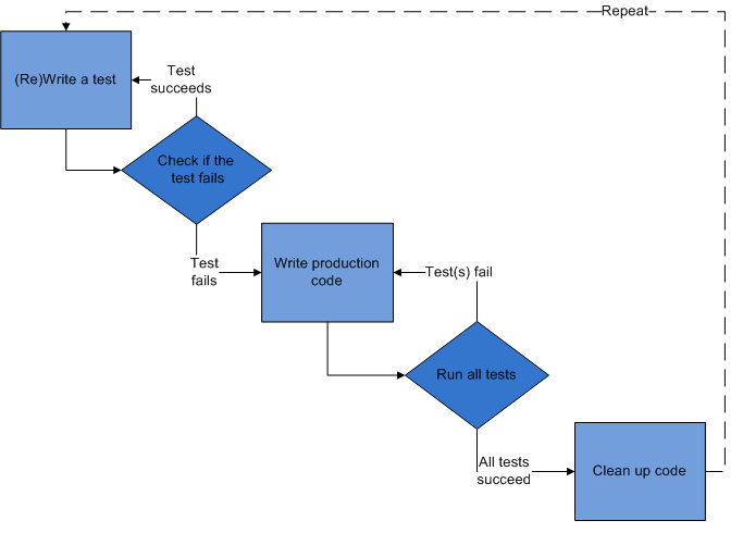
- Write a Test
-
In TDD, each new feature begins with writing a test — it is the first
step in adding new functionality to our software. This test must
inevitably fail because it is written before the feature has been
implemented — if it does not fail, then either the new feature
already exists or the test is defective. Writing a test could also
imply a variant, or modification of an existing test. This is a
differentiating property of TDD versus writing unit tests after the
code is written: it makes us focus on the requirements before writing
the code, a subtle but important difference.
-
To write a test, we must clearly understand the feature's
specification and requirements. This can be accomplish through use of
design documents, particularly the URD (User Requirements Document).
Each test needs to pass source code checkers and comply with best
practices such as coding style (a test is just code after all...).
- Check if Test fails
-
This validates that a test is working correctly and that the new test
does not mistakenly pass without requiring any new code. This step
also tests the test itself, in the negative sense: it rules out the
possibility that the new test will always pass, and therefore be
worthless. The new test should also fail for the expected reason. This
increases confidence (although it does not entirely guarantee) that it
is testing the right thing, and will pass only in intended cases.
- Write Production Code
-
Next we write code that will cause the test to pass. The new code
written at this stage will not be perfect and may, for example, pass
the test in an inelegant way — we want to make sure however that even
at this early stage our code passes source code checkers and complies
with best practices such as coding style. It is important that the
code written is only designed to pass the test i.e. no additional
functionality should be added.
- Run all Tests
-
With the new code written, we run all our tests again. If all tests
pass, we can be confident that the code we wrote adds the
features/functionality as described in our design documents e.g. the
URD. This is a good point from which to begin the final step of the
TDD cycle...
- Clean Up Code
-
Now the code can be cleaned up as necessary. By re-running tests
(including code coverage analyzers) we can also be confident that code
refactoring is not causing regressions of existing
functionality/features. Cleaning up also means removing duplication
and/or removing orphaned/unused production code — in this case,
however, it also applies to removing any duplication in test and
production code.
- Repeat
-
A new cycle starts when we start writing another test. The size of
each cycle should always be small — whatever limit we hit first: ~15
lines of code, ~30 minutes worth of work...
-
If new code does not rapidly satisfy a new test, or other tests fail
unexpectedly, we should undo or revert to debugging.
Continuous integration/deployment often helps in providing revertible
checkpoints.
Unit Testing
WRITEME
Integration Testing
System Testing
Source Code Checker
We use source code checkers for static source code checks i.e. to test
whether or not code is in compliance with a predefined set of rules
and best practices such as coding style. This might happen several
times before code makes it to production — the developer would
manually run a source code checker on the code he just wrote before he
checks it into the source code repository, in addition our continuous
integration/deployment system would run those checks again
automatically for any new commit that passes trough on the way to
production.
The use of analytical methods to check source code in order to detect
software defects and improve quality in general is nothing new — it
is the most basic thing to do for quality assurance and should be a
given for any software project.
pep8
pep8 checks code for PEP 8 compliance. We can run it manually or have
it run automatically by our continuous integration/deployment setup.
Our tests and pdb support it. It can be installed using aptitude
install pep8 or with PIP using pip install pep8.
PyChecker
In addition to the bug-checking that PyChecker performs, Pylint offers
some additional features such as checking line length, whether
variable names are well-formed according to our coding standard,
whether declared interfaces are fully implemented...
Pylint
This one is a very good compliment to pep8 and I would recommend it as
it really improves code quality right away. As for pep8, we can run it
manually or have it run automatically by our continuous
integration/deployment setup.
I ended up using them over others (pychecker, pyflakes...) because
pep8 and pylint work fine with GNU Emacs, they are well maintained,
feature-rich, and integrate well with other tools from the Python
ecosystem. Pylint can be installed using pip install pylint
pylint-i18n or via APT.
py.test
py.test can be used for unit testing, integration testing and
system testing — one tool to test our software end-to-end.
- http://sontek.net/writing-tests-for-pyramid-and-sqlalchemy
- with py.test, when you are running in parallel mode, the
pytest_sessionstart hook gets fired for each node, so we check
that we are on the master node.
- tests are run in the order we specify them, making tests both
deterministic and predictable
- we can ask py.test to abort on first error encountered using -x
option
- running tests will start immediately upon collecting them
- we can start py.test in daemon mode, which will then constantly
monitor our source code for changes and run tests automatically
WRITEME
Assertions
py.test does assertion introspection i.e. by default we do not get
Python's default assert semantics — py.test rewrites assert
statements in test code on import.
py.test only rewrites test code directly discovered by its test
collection process. This means that assert statements in supporting
code which is not itself test code will not be rewritten. Also, for
assert statements in test code with a manually provided message i.e.
assert expr, message, no assertion introspection takes place meaning
that the manually provided message will be rendered in tracebacks.
Assertion Introspection Methods
py.test has three assertion introspection methods: plain, reinterp and
rewrite (default). If we want Python's standard assert semantics even
for assert in test code then we can use --assert=plain
which results in an AssertionError exception instead of py.test's much
more informative default output from rewriting assert statements.
Funcargs
built-in Funcargs
- http://pytest.org/latest/tmpdir.html
Mysetup Pattern
- Decouple Test Code from Fixtures
- the mysetup factory is a funcarg; a helper/fixture object... a
class/type we instantiate
- have a
conftest.py to separate test code from fixtures
Parametrized Testing
pytest-cov
pytest-pep8
- does it just check test code for PEP 8 compliance or does it check
production code as well?
Miscellaneous
Debugging
Debugging is the process of trying to find out why a certain technical
system does not show a certain expected behavior and/or fails to
produce any reasonable result at all. The inverse is true as well...
debugging is sometimes used to verify expected outcome.

While the main purpose of debugging certainly is about tracking down
errors and/or unexpected behavior, debugging is also very good in
terms of educating ourselves because it allows us to look behind the
curtain of what Python is doing at any moment — what the names are it
is currently dealing with, what codepath that lead to a certain
subroutine... good stuff!
Our tool of choice is pdb, the module that defines an interactive
source code debugger for Python programs and which is shipped as part
of Python's standard library.
pdb supports setting breakpoints, stepping through source code line by
line, inspecting stack frames, source code listing, evaluation of
arbitrary Python code in the context of any stack frame, post-mortem
debugging and then some more... It can be called from a running
program or dropped into on error when running tests.
pdb is also extensible as it defines the class/type Pdb which we can
use to build upon. It is overall a very powerful tool, not just by
itself but also because it integrates nicely with other tools from the
Python ecosystem. Let us have a first look at it now:
>>> import sys
>>> 'pdb' in sys.builtin_module_names
False # pdb is not a built-in module but
>>> import pdb
>>> pdb.__file__
'/home/sa/0/cpython3.3/lib/python3.3/pdb.py' # shipped as part of the standard library
>>> import os
>>> os.path.dirname(pdb.__file__) in sys.path # pdb lives on sys.path per default so import is easy
True
>>> pdb.__all__ # pdb's public API
['run',
'pm',
'Pdb', # class Pdb which can be used to extend pdb
'runeval',
'runctx',
'runcall',
'set_trace',
'post_mortem',
'help']
>>>
Starting pdb
As mentioned, there are a few ways to start the debugger...
Command Line
The first one is to simply start it from the command line and feed it
some piece of Python source code. Let us draft something quickly which
we can feed to pdb:
#!/usr/bin/env python
class Foo:
def __init__(self, num_loops):
self.count = num_loops
def go(self):
for i in range(self.count):
print(i)
return
if __name__ == '__main__':
Foo(5).go()
and then feed it to pdb on the command line
(py33) sa@wks:~/0/py33$ python -m pdb pdb0.py
> /home/sa/0/py33/pdb0.py(4)<module>()
-> class Foo:
(Pdb) list
1 #!/usr/bin/env python
2
3
4 -> class Foo: # pdb pauses on encounter of the first statement/expression
5
6 def __init__(self, num_loops):
7 self.count = num_loops
8
9 def go(self):
10 for i in range(self.count):
11 print(i)
(Pdb)
Running pdb from the command line causes it to load our source file
pdb0.py and stop execution at the first statement or expression it
finds. In this case, it stops before evaluating the definition of the
class/type Foo on line 4. We then use the list command to show some
source code in context of where pdb currently pauses and waits for
further instructions from us — the current line of execution in the
current frame is always indicated by ->.
Interactive Interpreter Session
We can also start pdb from an interactive interpreter session:
>>> import pdb
>>> import pdb0
>>> pdb.run('pdb0.Foo(5).go()')
> <string>(1)<module>()->None
(Pdb) step
--Call--
> /home/sa/0/py33/pdb0.py(6)__init__()
-> def __init__(self, num_loops):
(Pdb) list
1 #!/usr/bin/env python
2
3
4 class Foo:
5
6 -> def __init__(self, num_loops):
7 self.count = num_loops
8
9 def go(self):
10 for i in range(self.count):
11 print(i)
(Pdb) quit
>>>
Many Pythoneers use this workflow with the interactive interpreter
while developing early versions of their software because it lets them
experiment more interactively without the save/run/repeat cycle
otherwise needed. As can be seen, to run pdb from within an
interactive interpreter session run(), runcall() or runeval() can be
used.
The argument to run() is a statement that can be evaluated by the
Python interpreter. pdb will parse it, then pause execution just
before the first statement/expression on the given codepath evaluates.
In our case that would again be the class definition of Foo. We use
step to move to the next line and list to provide ourselves with some
context around the line where pdb currently pauses execution
(indicated by ->).
From a running Program
Both of the previous examples assume we want to start the debugger at
the beginning of our program. For a long-running process where the
problem appears much later during program execution, it is more
convenient to start the debugger from inside our running program using
set_trace() which enters pdb at the calling stack frame:
(py33) sa@wks:~/0/py33$ cat pdb0.py
#!/usr/bin/env python
import pdb
class Foo:
def __init__(self, num_loops):
self.count = num_loops
def go(self):
for i in range(self.count):
pdb.set_trace()
print(i)
return
if __name__ == '__main__':
Foo(5).go()
(py33) sa@wks:~/0/py33$ chmod 755 pdb0.py
(py33) sa@wks:~/0/py33$ ./pdb0.py
> /home/sa/0/py33/pdb0.py(14)go()
-> print(i)
(Pdb) list
9 self.count = num_loops
10
11 def go(self):
12 for i in range(self.count):
13 pdb.set_trace()
14 -> print(i)
15 return
16
17
18 if __name__ == '__main__':
19 Foo(5).go()
(Pdb) quit
(py33) sa@wks:~/0/py33$
Line 13 of the sample script triggers pdb at that point in execution.
set_trace() is just a Python function which allows us to call it at
any point in our program. This lets us drop into pdb based on
conditions inside our program, including from an exception handler or
via a specific branch of a control statement.
After a Failure
Debugging a failure after a program terminates is called post-mortem
debugging. pdb supports post-mortem debugging through the pm() and
post_mortem() functions:
(py33) sa@wks:~/0/py33$ cat pdb0.py
#!/usr/bin/env python
class Foo:
def __init__(self, num_loops):
self.count = num_loops
def go(self):
for i in range(foobarbaz):
print(i)
return
if __name__ == '__main__':
Foo(5).go()
(py33) sa@wks:~/0/py33$ python
>>> import pdb0
>>> pdb0.Foo(3).go()
Traceback (most recent call last):
File "<input>", line 1, in <module>
File "pdb0.py", line 10, in go
for i in range(foobarbaz):
NameError: global name 'foobarbaz' is not defined
>>> import pdb
>>> pdb.pm()
> /home/sa/0/py33/pdb0.py(10)go()
-> for i in range(foobarbaz):
(Pdb) print foobarbaz
NameError: name 'foobarbaz' is not defined
(Pdb) list
5
6 def __init__(self, num_loops):
7 self.count = num_loops
8
9 def go(self):
10 -> for i in range(foobarbaz):
11 print(i)
12 return
13
14
15 if __name__ == '__main__':
(Pdb)
Here the incorrect foobarbaz on line 10 triggers a NameError
exception, causing execution to stop. pm() looks for the active
traceback and starts pdb at the point on the call stack where the
exception occurred.
Dropping into pdb when running Tests
We are going to use py.test because it is the most sophisticated tool
out there:
(py33) sa@wks:~/0/py33$ pip freeze | grep test
pytest==2.2.0
pytest-pep8==0.7
(py33) sa@wks:~/0/py33$ (py33) sa@wks:~/0/py33$ py.test --pdb pdb0.py
====================== test session starts ======================
platform linux -- Python 3.3.0 -- pytest-2.2.0
collected 1 items
pdb0.py
>>>>>>>>>>>>>>>>>>>>>>>>>>> traceback >>>>>>>>>>>>>>>>>>>>>>>>>>>
def test_go():
> Foo(5).go()
pdb0.py:16:
_ _ _ _ _ _ _ _ _ _ _ _ _ _ _ _ _ _ _ _ _ _ _ _ _ _ _ _ _ _ _ _ _
self = <pdb0.Foo object at 0x7f91400e3290>
def go(self):
> for i in range(foobarbaz):
E NameError: global name 'foobarbaz' is not defined
pdb0.py:10: NameError
>>>>>>>>>>>>>>>>>>>>>>>>> entering PDB >>>>>>>>>>>>>>>>>>>>>>>>>>
> /home/sa/0/py33/pdb0.py(10)go()
-> for i in range(foobarbaz):
(Pdb) list 3, 20
3
4 class Foo:
5
6 def __init__(self, num_loops):
7 self.count = num_loops
8
9 def go(self):
10 -> for i in range(foobarbaz):
11 print(i)
12 return
13
14
15 def test_go():
16 Foo(5).go()
17
18
19 if __name__ == '__main__':
20 Foo(5).go()
(Pdb) quit
F
=================== 1 failed in 5.82 seconds ====================
(py33) sa@wks:~/0/py33$
py.test looks for functions/methods prefixed with test_, collects them
and subsequently runs them. We would usually gather test_* functions
inside a separate test module but for now we put test_go() inside
pdb0.py for convenience and simplicity.
py.test runs test_go() which of course triggers the error on line 10.
py.test then does its usual magic and finally drops into pdb
(entering PDB) because we provided the --pdb argument when we
started py.test on pdb0.py.
The same semantics that apply to using pdb.set_trace() also apply to
pytest.set_trace() with the addition that we drop into pdb when we run
our tests using py.test (if we would use pdb.set_trace() in line 13
then we would not drop into pdb when using py.test):
(py33) sa@wks:~/0/py33$ cat pdb0.py
#!/usr/bin/env python
import pytest # no need for an additional import pdb
class Foo:
def __init__(self, num_loops):
self.count = num_loops
def go(self):
for i in range(self.count):
pytest.set_trace()
print(i)
return
def test_go():
Foo(5).go()
if __name__ == '__main__':
Foo(5).go()
(py33) sa@wks:~/0/py33$ py.test --pep8 pdb0.py
=========================== test session starts ============================
platform linux -- Python 3.3.0 -- pytest-2.2.0
pep8 ignore opts: (performing all available checks)
collected 2 items
pdb0.py .
>>>>>>>>>>>>>>>>> PDB set_trace (IO-capturing turned off) >>>>>>>>>>>>>>>>>>
> /home/sa/0/py33/pdb0.py(14)go()
-> print(i)
(Pdb) list
9 self.count = num_loops
10
11 def go(self):
12 for i in range(self.count):
13 pytest.set_trace()
14 -> print(i)
15 return
16
17
18 def test_go():
19 Foo(5).go()
(Pdb) print i, self.count
(0, 5)
(Pdb) quit
(py33) sa@wks:~/0/py33$
Interactive Commands
pdb is designed to be easy to use interactively. We can interact with
it using a small command language (list, quit...) that lets us move
around the call stack, examine and change values, control how pdb
executes our programs and much more. pdb uses readline to accept
commands which is why Python should have been build with readline
support:
>>> import readline
>>> readline.__file__
'/home/sa/0/py33/lib/python3.3/lib-dynload/readline.cpython-33m.so'
>>>
Getting Help
Once at the pdb prompt we can then use help to show us the available
commands. One thing important to note is that most commands have a
long and a short version e.g. typing print or p actually runs the same
command:
(py33) sa@wks:~/0/py33$ python pdb0.py
> /home/sa/0/py33/pdb0.py(14)go()
-> print(i)
(Pdb) help
Documented commands (type help <topic>):
========================================
EOF cl disable interact next return u where
a clear display j p retval unalias
alias commands down jump pp run undisplay
args condition enable l print rv unt
b cont exit list q s until
break continue h ll quit source up
bt d help longlist r step w
c debug ignore n restart tbreak whatis
Miscellaneous help topics:
==========================
pdb exec
(Pdb)
We can also get to certain help topics by using help <topic> such as:
(Pdb) help until
unt(il) [lineno]
Without argument, continue execution until the line with a
number greater than the current one is reached. With a line
number, continue execution until a line with a number greater
or equal to that is reached. In both cases, also stop when
the current frame returns.
(Pdb) help exec
(!) statement
Execute the (one-line) statement in the context of the current
stack frame. The exclamation point can be omitted unless the
first word of the statement resembles a debugger command. To
assign to a global variable you must always prefix the command
with a 'global' command, e.g.:
(Pdb) global list_options; list_options = ['-l']
(Pdb)
(Pdb)
Navigating the Execution Stack
Unless the command was list, entering a blank line re-runs the
previous command again:
(Pdb) w
/home/sa/0/py33/pdb0.py(23)<module>()
-> Foo(5).go()
> /home/sa/0/py33/pdb0.py(14)go()
-> print(i)
(Pdb) # runs w/where again
/home/sa/0/py33/pdb0.py(23)<module>()
-> Foo(5).go()
> /home/sa/0/py33/pdb0.py(14)go()
-> print(i)
(Pdb) list
9 self.count = num_loops
10
11 def go(self):
12 for i in range(self.count):
13 pdb.set_trace()
14 -> print(i)
15 return
16
17
18 if __name__ == '__main__':
19 Foo(5).go()
(Pdb) # does not run l/list again
[EOF]
(Pdb)
As can be seen, at any point while pdb is running we can use where to
find out exactly what line is being executed and where on the call
stack we are. In this case, the module pdb0.py line 14 in the go()
method. where can prove invaluable when debugging bigger programs that
run on a bunch of libraries — a situation where we literally have to
go down the rabbit hole when we need to get at the bottom of things.
list can be used without arguments in which case it displays 11 lines
around the current line (five before and five after). Using list with
a single numerical argument (e.g. lists 33) lists lines around that
line instead of the current line, and providing two arguments e.g.
list 4, 33 would list lines 4 to 33. In all cases -> points at the
current execution point (beginning of a line containing a
statement/expression).
Moving up/down the Call Stack
If up/down the call stack sounds confusing then we can just think
about it as back and forth in time between the point in time where
Python starts executing our program and the point in time where we
actually drop into pdb.
Two very handy commands in addition to where are up and down (or u and
d respectively) as they allow us to move up and down the call stack —
up for older and down for newer frames as growth happens top-down:
(Pdb) where # let us have a look at the call stack
/home/sa/0/py33/pdb0.py(19)<module>()
-> Foo(5).go() # first (topmost) stack frame on the call stack
> /home/sa/0/py33/pdb0.py(14)go()
-> print(i) # second stack frame
(Pdb) l
9 self.count = num_loops
10
11 def go(self):
12 for i in range(self.count):
13 pdb.set_trace()
14 -> print(i) # execution pauses after the pdb.set_trace() line
15 return
16
17
18 if __name__ == '__main__':
19 Foo(5).go()
(Pdb) up # move to older stack frame (upwards the call stack)
> /home/sa/0/py33/pdb0.py(19)<module>()
-> Foo(5).go()
(Pdb) l
14 print(i)
15 return
16
17
18 if __name__ == '__main__':
19 -> Foo(5).go() # first stack frame
[EOF]
(Pdb) down # move to newer stack frame again (downwards the call stack)
> /home/sa/0/py33/pdb0.py(14)go()
-> print(i)
(Pdb) l
9 self.count = num_loops
10
11 def go(self):
12 for i in range(self.count):
13 pdb.set_trace()
14 -> print(i) # back on second stack frame
15 return
16
17
18 if __name__ == '__main__':
19 Foo(5).go()
(Pdb)
Examining Variables on the Call Stack
The args command prints all of the arguments to the function/method
active in the current stack frame. This example also uses the
recursive function foo() to show what a stack looks like when where is
used:
(py33) sa@wks:~/0/py33$ cat pdb1.py
#!/usr/bin/env python
import pdb
def foo(n=5, output="to be printed"):
if n > 0:
foo(n - 1)
else:
pdb.set_trace()
print(output)
return
if __name__ == '__main__':
foo()
(py33) sa@wks:~/0/py33$ python pdb1.py
> /home/sa/0/py33/pdb1.py(11)foo()
-> print(output)
(Pdb) where
/home/sa/0/py33/pdb1.py(17)<module>()
-> foo()
/home/sa/0/py33/pdb1.py(8)foo()
-> foo(n - 1)
/home/sa/0/py33/pdb1.py(8)foo()
-> foo(n - 1)
/home/sa/0/py33/pdb1.py(8)foo()
-> foo(n - 1)
/home/sa/0/py33/pdb1.py(8)foo()
-> foo(n - 1)
/home/sa/0/py33/pdb1.py(8)foo()
-> foo(n - 1)
> /home/sa/0/py33/pdb1.py(11)foo()
-> print(output)
As can be seen, execution pauses after the pdb.set_trace() line,
nothing new here. What is interesting is that we can see that in order
to get there the call stack grew by 7 frames. Let us have a look at
the arguments now, both, in the current stack frame and the one before
the current one:
(Pdb) args
n = 0
output = 'to be printed'
(Pdb) up # going back in time, up the call stack
> /home/sa/0/py33/pdb1.py(8)foo()
-> foo(n - 1)
(Pdb) args
n = 1
output = 'to be printed'
(Pdb) print n # print evaluates an expression using the current frame variables/state
1
(Pdb) print n + 4
5
(Pdb) down # going forward in time, down the call stack
> /home/sa/0/py33/pdb1.py(11)foo()
-> print(output) # back at the frame where execution initially paused
The print command evaluates an expression given as argument and prints
the result (there is also pp which semantically is the same as print
except it used Python's pprint module, therefore might be the better
fit to use when looking at complex/nested data structures).
We could also use Python's print() function, but that is passed
through to the interpreter to be executed rather than running as
inside pdb. Similarly, prefixing an expression with ! passes it to the
Python interpreter to be evaluated. We can use this feature to execute
arbitrary Python statements, including modifying variables. Let us
change the value of output before letting pdb continue executing the
program. The next statement after the call to set_trace() prints the
value of output, showing the modified value:
(pdb) print(sys.version[:3]) # pass through to the interpreter
'3.3'
(Pdb) !output # pass through to the interpreter and evaluate
'to be printed'
(Pdb) !output = "but I want THIS to be printed..."
(Pdb) l
6 def foo(n=5, output="to be printed"):
7 if n > 0:
8 foo(n - 1)
9 else:
10 pdb.set_trace()
11 -> print(output)
12
13 return
14
15
16 if __name__ == '__main__':
(Pdb) step # step through line 11 (execute it)
but I want THIS to be printed...
> /home/sa/0/py33/pdb1.py(13)foo()
-> return
(Pdb)
Stepping through a Program
In addition to navigating up and down the call stack using up and down
when the program is paused, we can also step through the program past
the point where execution pauses and we drop into pdb. Commands to do
so are step, next, until and return:
(py33) sa@wks:~/0/py33$ cat pdb2.py
#!/usr/bin/env python
import pdb
def faz(n):
for i in range(n):
j = i * n
print(i, j)
return
if __name__ == '__main__':
pdb.set_trace()
faz(5)
(py33) sa@wks:~/0/py33$ python pdb2.py
> /home/sa/0/py33/pdb2.py(15)<module>()
-> faz(5)
(Pdb) l
10 return
11
12
13 if __name__ == '__main__':
14 pdb.set_trace()
15 -> faz(5)
[EOF]
(Pdb) s
--Call--
> /home/sa/0/py33/pdb2.py(6)faz()
-> def faz(n):
(Pdb) l
1 #!/usr/bin/env python
2
3 import pdb
4
5
6 -> def faz(n):
7 for i in range(n):
8 j = i * n
9 print(i, j)
10 return
11
(Pdb) s
> /home/sa/0/py33/pdb2.py(7)faz()
-> for i in range(n): # third execution point after dropping into pdb
(Pdb) # hitting enter repeats the last command (step)
> /home/sa/0/py33/pdb2.py(8)faz()
-> j = i * n
(Pdb) p i, n
(0, 5)
As we already know, the call to set_trace() drops us into pdb and
pauses execution right after the callout to set_trace() (beginning of
line 15 in our case). We can then use step to execute the current line
and then stop at the next execution point — either the first
statement of a function/method being called (--Call--) or the next
line of the current function/method.
step is the slowest way of moving along the codepath of our program as
it literally enters into any function/method and follows along any
callout to any library we use in our program. We can do it faster
using next:
(Pdb) u
> /home/sa/0/py33/pdb2.py(15)<module>()
-> faz(5)
(Pdb) next
0 0
1 5
2 10
3 15
4 20
--Return--
> /home/sa/0/py33/pdb2.py(15)<module>()->None
-> faz(5)
(Pdb) s
(py33) sa@wks:~/0/py33$
As can be seen, we first went up the call stack again using up (or u
for that matter). We are then paused at the beginning of line 15
again, right before calling faz(). What next does compared to step is
not enter into the function/method called from the current execution
point but rather executing it at full-speed, only stopping at the next
line inside the current function/method. In our current case the
codepath goes through faz() and thus the for loop, looping over
print(i, j) five times and printing the values and then returning and
pausing again at the beginning of line 15, right before the next
execution point.
Something in between step and next is return as it allows us to enter
into a function/method, step a few times and then continue execution
until the current function/method returns:
(py33) sa@wks:~/0/py33$ python pdb2.py
> /home/sa/0/py33/pdb2.py(15)<module>()
-> faz(5)
(Pdb) s # we make a step
--Call--
> /home/sa/0/py33/pdb2.py(6)faz()
-> def faz(n):
(Pdb) s # another step
> /home/sa/0/py33/pdb2.py(7)faz()
-> for i in range(n):
(Pdb) p n # look at values in the current frame
5 # maybe found what we were looking for
(Pdb) return # and thus skip forward
0 0
1 5
2 10
3 15
4 20
--Return--
> /home/sa/0/py33/pdb2.py(10)faz()->None
-> return # explicit return i.e. function returns here
(Pdb) w
/home/sa/0/py33/pdb2.py(15)<module>()
-> faz(5)
> /home/sa/0/py33/pdb2.py(10)faz()->None
-> return
(Pdb)
(py33) sa@wks:~/0/py33$
until is semantically close to next and return but more
flexible/powerful because it allows us to specify a line number up to
which we want execution to run before it is paused again. If we do not
specify a line number then execution will run until it reaches a line
number greater than the current one:
(py33) sa@wks:~/0/py33$ cat pdb3.py
#!/usr/bin/env python
import pdb
def bar(i, n):
return i * n
def baz(n):
for i in range(n):
j = bar(i, n)
print(i, j)
return
if __name__ == '__main__':
pdb.set_trace()
baz(5)
(py33) sa@wks:~/0/py33$ python pdb3.py
> /home/sa/0/py33/pdb3.py(19)<module>()
-> baz(5)
(Pdb) s
--Call--
> /home/sa/0/py33/pdb3.py(10)baz()
-> def baz(n):
(Pdb) l
5
6 def bar(i, n):
7 return i * n
8
9
10 -> def baz(n):
11 for i in range(n):
12 j = bar(i, n)
13 print(i, j)
14 return
15
(Pdb) until 13 # execute until line 13
> /home/sa/0/py33/pdb3.py(13)baz()
-> print(i, j)
(Pdb) p i, j, n
(0, 0, 5)
(Pdb) s
0 0
> /home/sa/0/py33/pdb3.py(11)baz()
-> for i in range(n):
(Pdb) s
> /home/sa/0/py33/pdb3.py(12)baz()
-> j = bar(i, n)
(Pdb) s
--Call--
> /home/sa/0/py33/pdb3.py(6)bar()
-> def bar(i, n):
(Pdb) l
1 #!/usr/bin/env python
2
3 import pdb
4
5
6 -> def bar(i, n):
7 return i * n
8
9
10 def baz(n):
11 for i in range(n):
(Pdb) r
--Return--
> /home/sa/0/py33/pdb3.py(7)bar()->5 # return value is 5
-> return i * n
(Pdb) s
> /home/sa/0/py33/pdb3.py(13)baz()
-> print(i, j)
(Pdb) p i, j, n
(1, 5, 5)
(Pdb) w
/home/sa/0/py33/pdb3.py(19)<module>()
-> baz(5)
> /home/sa/0/py33/pdb3.py(13)baz()
-> print(i, j)
(Pdb) l
8
9
10 def baz(n):
11 for i in range(n):
12 j = bar(i, n)
13 -> print(i, j)
14 return
15
16
17 if __name__ == '__main__':
18 pdb.set_trace()
(Pdb) until # continue execution until the line with a number greater than the current one is reached
1 5
2 10
3 15
4 20
> /home/sa/0/py33/pdb3.py(14)baz()
-> return
(Pdb) s
--Return--
> /home/sa/0/py33/pdb3.py(14)baz()->None
-> return # next line after the for loop is exhausted
(Pdb) s
--Return--
> /home/sa/0/py33/pdb3.py(19)<module>()->None
-> baz(5)
(Pdb) l
14 return
15
16
17 if __name__ == '__main__':
18 pdb.set_trace()
19 -> baz(5)
[EOF]
(Pdb) s
(py33) sa@wks:~/0/py33$
Breakpoints
The most powerful way of stepping trough our programs is done using
so-called breakpoints: As programs grow longer, even using next and
until will become a tedious thing to do.
A better solution is to let the program execute until it reaches a
point where we want execution to pause and hand control over to pdb.
We could use set_trace() to drop us into pdb, but that only works if
there is only one point where we want to pause execution...
It is more convenient to run our program through pdb and tell it where
to pause execution using so-called breakpoints. pdb would then pause
execution at the line before a breakpoint and drop us into the pdb
prompt:
(py33) sa@wks:~/0/py33$ cat pdb4.py
#!/usr/bin/env python
def calc(i, n):
bar = i * n
print('bar =', bar)
if bar > 0:
print('bar is positive')
return bar
def foo(n):
for i in range(n):
print('i =', i)
bar = calc(i, n)
return
if __name__ == '__main__':
foo(5)
(py33) sa@wks:~/0/py33$ python -m pdb pdb4.py
> /home/sa/0/py33/pdb4.py(4)<module>()
-> def calc(i, n):
(Pdb) l
1 #!/usr/bin/env python
2
3
4 -> def calc(i, n): # pdb pauses on encounter of the first statement/expression
5 bar = i * n
6 print('bar =', bar)
7 if bar > 0:
8 print('bar is positive')
9
10 return bar
11
(Pdb) w
/home/sa/0/cpython3.3/lib/python3.3/bdb.py(392)run()
-> exec(cmd, globals, locals)
<string>(1)<module>()
> /home/sa/0/py33/pdb4.py(4)<module>()
-> def calc(i, n):
(Pdb) break 8 # set breakpoint using a line number
Breakpoint 1 at /home/sa/0/py33/pdb4.py:8
(Pdb) continue # keep executing until the next breakpoint
i = 0
bar = 0
i = 1
bar = 5
> /home/sa/0/py33/pdb4.py(8)calc()
-> print('bar is positive')
(Pdb)
There are several options to break — we can specify a line number
(above), a file, or a function/method (below):
(py33) sa@wks:~/0/py33$ python -m pdb pdb4.py
> /home/sa/0/py33/pdb4.py(4)<module>()
-> def calc(i, n):
(Pdb) break calc # using a function name to set the breakpoint
Breakpoint 1 at /home/sa/0/py33/pdb4.py:4 # breakpoint with ID 1
(Pdb) l
1 #!/usr/bin/env python
2
3
4 B-> def calc(i, n): # set breakpoint indicated by capital B
5 bar = i * n
6 print('bar =', bar)
7 if bar > 0:
8 print('bar is positive')
9
10 return bar
11
(Pdb) continue
i = 0
> /home/sa/0/py33/pdb4.py(5)calc()
-> bar = i * n
(Pdb) w
/home/sa/0/cpython3.3/lib/python3.3/bdb.py(392)run()
-> exec(cmd, globals, locals)
<string>(1)<module>()
/home/sa/0/py33/pdb4.py(21)<module>()
-> foo(5)
/home/sa/0/py33/pdb4.py(16)foo()
-> bar = calc(i, n)
> /home/sa/0/py33/pdb4.py(5)calc()
-> bar = i * n
(Pdb)
continue tells pdb to keep executing the program until it encounters
the next breakpoint. With the first example where we set the
breakpoint at line 8, the codepath runs through the first iteration of
the for loop in foo(), goes into calc() where it does not encounter
the breakpoint we set so another iteration through the for loop and
calc() happens before it pauses inside calc() during the second
iteration at line 8, just where we set the breakpoint...
Managing Breakpoints
As each new breakpoint is added, it is assigned a numerical
identifier. These IDs can then be used to enable, disable, and clear
the breakpoints interactively.
The debugging session below sets two breakpoints, then disables one.
The program is run until the remaining breakpoint is encountered, and
then the other breakpoint is turned back on with the enable command
before execution continues. At the end we decide to clear/delete the
breakpoint we just re-enabled because we might have concluded it was
superfluous anyway — other breakpoints retain their original IDs and
are not renumbered:
(py33) sa@wks:~/0/py33$ python -m pdb pdb4.py
> /home/sa/0/py33/pdb4.py(4)<module>()
-> def calc(i, n): # pdb pauses on encounter of the first statement/expression
(Pdb) l
1 #!/usr/bin/env python
2
3
4 -> def calc(i, n):
5 bar = i * n
6 print('bar =', bar)
7 if bar > 0:
8 print('bar is positive')
9
10 return bar
11
(Pdb) break calc
Breakpoint 1 at /home/sa/0/py33/pdb4.py:4
(Pdb) break 8
Breakpoint 2 at /home/sa/0/py33/pdb4.py:8
(Pdb) break # list breakpoints
Num Type Disp Enb Where
1 breakpoint keep yes at /home/sa/0/py33/pdb4.py:4
2 breakpoint keep yes at /home/sa/0/py33/pdb4.py:8
(Pdb) l 1, 10
1 #!/usr/bin/env python
2
3
4 B-> def calc(i, n): # execution currently paused at breakpoint with ID 1
5 bar = i * n
6 print('bar =', bar)
7 if bar > 0:
8 B print('bar is positive')
9
10 return bar
(Pdb) disable 1 # disable a breakpoint
Disabled breakpoint 1 at /home/sa/0/py33/pdb4.py:4
(Pdb) break
Num Type Disp Enb Where
1 breakpoint keep no at /home/sa/0/py33/pdb4.py:4
2 breakpoint keep yes at /home/sa/0/py33/pdb4.py:8
(Pdb) continue
i = 0
bar = 0
i = 1
bar = 5
> /home/sa/0/py33/pdb4.py(8)calc()
-> print('bar is positive')
(Pdb) break
Num Type Disp Enb Where
1 breakpoint keep no at /home/sa/0/py33/pdb4.py:4
2 breakpoint keep yes at /home/sa/0/py33/pdb4.py:8
breakpoint already hit 1 time # we hit breakpoint with ID 2 once already
(Pdb) enable 1 # enable a disables breakpoint
Enabled breakpoint 1 at /home/sa/0/py33/pdb4.py:4
(Pdb) break
Num Type Disp Enb Where
1 breakpoint keep yes at /home/sa/0/py33/pdb4.py:4 # marked non-temporary (keep)
2 breakpoint keep yes at /home/sa/0/py33/pdb4.py:8
breakpoint already hit 1 time
(Pdb) w
/home/sa/0/cpython3.3/lib/python3.3/bdb.py(392)run()
-> exec(cmd, globals, locals)
<string>(1)<module>()
/home/sa/0/py33/pdb4.py(21)<module>()
-> foo(5)
/home/sa/0/py33/pdb4.py(16)foo()
-> bar = calc(i, n)
> /home/sa/0/py33/pdb4.py(8)calc()
-> print('bar is positive')
(Pdb) l
3
4 B def calc(i, n):
5 bar = i * n
6 print('bar =', bar)
7 if bar > 0:
8 B-> print('bar is positive')
9
10 return bar
11
12
13 def foo(n):
(Pdb) clear 1 # delete/clear breakpoint with ID 1
Deleted breakpoint 1 at /home/sa/0/py33/pdb4.py:4
(Pdb) break
Num Type Disp Enb Where
2 breakpoint keep yes at /home/sa/0/py33/pdb4.py:8
breakpoint already hit 1 time
(Pdb) l 1, 10
1 #!/usr/bin/env python
2
3
4 def calc(i, n):
5 bar = i * n
6 print('bar =', bar)
7 if bar > 0:
8 B-> print('bar is positive')
9
10 return bar
(Pdb)
Temporary Breakpoints
A temporary breakpoint is automatically cleared the first time program
execution hits it. Using a temporary breakpoint lets us reach a
particular spot in the program flow quickly, just as with a regular
breakpoint, but since it is cleared immediately it does not interfere
with subsequent progress if that part of the program is run
repeatedly:
(py33) sa@wks:~/0/py33$ python -m pdb pdb4.py
> /home/sa/0/py33/pdb4.py(4)<module>()
-> def calc(i, n):
(Pdb) tbreak 8 # set temporary breakpoint at line 8
Breakpoint 1 at /home/sa/0/py33/pdb4.py:8
(Pdb) break
Num Type Disp Enb Where
1 breakpoint del yes at /home/sa/0/py33/pdb4.py:8 # marked temporary (del)
(Pdb) l
1 #!/usr/bin/env python
2
3
4 -> def calc(i, n):
5 bar = i * n
6 print('bar =', bar)
7 if bar > 0:
8 B print('bar is positive')
9
10 return bar
11
(Pdb) c
i = 0
bar = 0
i = 1
bar = 5
Deleted breakpoint 1 at /home/sa/0/py33/pdb4.py:8 # pdb deletes temporary breakpoint automatically
> /home/sa/0/py33/pdb4.py(8)calc()
-> print('bar is positive')
(Pdb) break # temporary breakpoint is gone
(Pdb) q
(py33) sa@wks:~/0/py33$
Conditional Breakpoints
Rather than enabling/disabling breakpoints manually we can use
conditional breakpoints which then gives us finer control over when
pdb pauses our program. Conditions can be applied to breakpoints so
that execution only pauses when those conditions are met. Conditional
breakpoints can be set in two ways:
- The first is to specify the condition when the breakpoint is set,
using
break. The condition argument must be an expression, using
values visible in the current stack frame where the breakpoint is
defined. If the expression evaluates to true, execution pauses at
the breakpoint.
- A condition can also be applied to an existing breakpoint using
the
condition command. The arguments are the breakpoint ID and the
expression.
(py33) sa@wks:~/0/py33$ python -m pdb pdb4.py
> /home/sa/0/py33/pdb4.py(4)<module>()
-> def calc(i, n):
(Pdb) break 5, i > 0 # set condition at the same time the breakpoint is set
Breakpoint 1 at /home/sa/0/py33/pdb4.py:5
(Pdb) break
Num Type Disp Enb Where
1 breakpoint keep yes at /home/sa/0/py33/pdb4.py:5
stop only if i > 0 # condition
(Pdb) l 1, 10
1 #!/usr/bin/env python
2
3
4 -> def calc(i, n):
5 B bar = i * n
6 print('bar =', bar)
7 if bar > 0:
8 print('bar is positive')
9
10 return bar
(Pdb) continue
i = 0
bar = 0
i = 1
> /home/sa/0/py33/pdb4.py(5)calc()
-> bar = i * n
(Pdb) l
1 #!/usr/bin/env python
2
3
4 def calc(i, n):
5 B-> bar = i * n
6 print('bar =', bar)
7 if bar > 0:
8 print('bar is positive')
9
10 return bar
11
(Pdb) p i, n
(1, 5)
(Pdb) condition 1 i > 4 # add condition to existing breakpoint with ID 1
New condition set for breakpoint 1.
(Pdb) break
Num Type Disp Enb Where
1 breakpoint keep yes at /home/sa/0/py33/pdb4.py:5
stop only if i > 4 # same breakpoint, new condition
breakpoint already hit 2 times
(Pdb) continue
bar = 5
bar is positive
i = 2
bar = 10
bar is positive
i = 3
bar = 15
bar is positive
i = 4
bar = 20
bar is positive
The program finished and will be restarted
> /home/sa/0/py33/pdb4.py(4)<module>()
-> def calc(i, n):
(Pdb) break
Num Type Disp Enb Where
1 breakpoint keep yes at /home/sa/0/py33/pdb4.py:5
stop only if i > 4
breakpoint already hit 5 times
(Pdb) q
(py33) sa@wks:~/0/py33$
Ignoring Breakpoints
Programs with a lot of looping or recursive calls to the same function
are often easier to debug by skipping ahead in the execution, instead
of watching every call or breakpoint. The ignore command tells pdb to
pass over a breakpoint without pausing. Each time processing
encounteres the breakpoint, it decrements the ignore counter. When the
counter is zero, the breakpoint is re-activated:
(py33) sa@wks:~/0/py33$ python -m pdb pdb4.py
> /home/sa/0/py33/pdb4.py(4)<module>()
-> def calc(i, n):
(Pdb) l
1 #!/usr/bin/env python
2
3
4 -> def calc(i, n):
5 bar = i * n
6 print('bar =', bar)
7 if bar > 0:
8 print('bar is positive')
9
10 return bar
11
(Pdb) break 8
Breakpoint 1 at /home/sa/0/py33/pdb4.py:8
(Pdb) ignore 1 2 # do not pause on the next two hits of breakpoint with ID 1
Will ignore next 2 crossings of breakpoint 1.
(Pdb) break
Num Type Disp Enb Where
1 breakpoint keep yes at /home/sa/0/py33/pdb4.py:8
ignore next 2 hits
(Pdb) continue
i = 0
bar = 0
i = 1
bar = 5
bar is positive
i = 2
bar = 10
bar is positive
i = 3
bar = 15
> /home/sa/0/py33/pdb4.py(8)calc()
-> print('bar is positive')
(Pdb) break
Num Type Disp Enb Where
1 breakpoint keep yes at /home/sa/0/py33/pdb4.py:8
breakpoint already hit 3 times
(Pdb) ignore 1 1
Will ignore next 1 crossing of breakpoint 1.
(Pdb) break
Num Type Disp Enb Where
1 breakpoint keep yes at /home/sa/0/py33/pdb4.py:8
ignore next 1 hits
breakpoint already hit 3 times
(Pdb) ignore 1 0 # explicitly resetting the ignore count to zero re-activates the breakpoint
Will stop next time breakpoint 1 is reached.
(Pdb) break
Num Type Disp Enb Where
1 breakpoint keep yes at /home/sa/0/py33/pdb4.py:8
breakpoint already hit 3 times
(Pdb) quit
(py33) sa@wks:~/0/py33$
Triggering Actions on a Breakpoint
In addition to the purely interactive mode, pdb supports basic
scripting. Using commands, we can define a series of interpreter
commands, including Python statements, to be executed when a specific
breakpoint is encountered.
After issuing the commands command with the breakpoint ID as argument,
the pdb prompt changes to (com). We then enter commands and/or Python
statements one at a time and issue the end command to save the script
which then returns us back to the main pdb prompt:
(py33) sa@wks:~/0/py33$ python -m pdb pdb4.py
> /home/sa/0/py33/pdb4.py(4)<module>()
-> def calc(i, n):
(Pdb) l
1 #!/usr/bin/env python
2
3
4 -> def calc(i, n):
5 bar = i * n
6 print('bar =', bar)
7 if bar > 0:
8 print('bar is positive')
9
10 return bar
11
(Pdb) break 5
Breakpoint 1 at /home/sa/0/py33/pdb4.py:5
(Pdb) commands 1 # start command session for breakpoint with ID 1
(com) print("i is {}".format(i)) # add Python statement
(com) end # end command session
(Pdb) continue
i = 0
'i is 0'
> /home/sa/0/py33/pdb4.py(5)calc()
-> bar = i * n
(Pdb) continue
bar = 0
i = 1
'i is 1'
> /home/sa/0/py33/pdb4.py(5)calc()
-> bar = i * n
(Pdb) break
Num Type Disp Enb Where
1 breakpoint keep yes at /home/sa/0/py33/pdb4.py:5
breakpoint already hit 2 times
(Pdb) condition 1 i > 2 # all other things work unchanged e.g. adding a condition
New condition set for breakpoint 1.
(Pdb) break
Num Type Disp Enb Where
1 breakpoint keep yes at /home/sa/0/py33/pdb4.py:5
stop only if i > 2
breakpoint already hit 2 times
(Pdb) continue
bar = 5
bar is positive
i = 2
bar = 10
bar is positive
i = 3
'i is 3'
> /home/sa/0/py33/pdb4.py(5)calc()
-> bar = i * n
(Pdb) quit
(py33) sa@wks:~/0/py33$
Restarting a Program
When pdb reaches the end of our program, it automatically restarts it.
We can also restart it explicitly without leaving pdb and thereby
losing breakpoints and other settings.
Running the below program to completion within the debugger prints the
name of the file, since no other arguments were given on the command
line:
(py33) sa@wks:~/0/py33$ cat pdb5.py
#!/usr/bin/env python
import sys
def foo():
print("Command line arguments: {}".format(sys.argv))
return
if __name__ == '__main__':
foo()
(py33) sa@wks:~/0/py33$ python -m pdb pdb5.py
> /home/sa/0/py33/pdb5.py(4)<module>() # first run through pdb5.py
-> import sys # pdb pauses on encounter of the first statement/expression
(Pdb) continue
Command line arguments: ['pdb5.py']
The program finished and will be restarted # pdb restarts a program automatically
> /home/sa/0/py33/pdb5.py(4)<module>() # second run through pdb5.py
-> import sys
The program can be restarted using run. Arguments passed to run are
parsed with shlex and passed to the program as though they were
command line arguments i.e. we can restart the program with different
settings:
(Pdb) run foo 2 "long argument..."
Restarting pdb5.py with arguments:
pdb5.py
> /home/sa/0/py33/pdb5.py(4)<module>()
-> import sys
(Pdb) continue
Command line arguments: ['pdb5.py', 'foo', '2', 'long argument...']
The program finished and will be restarted
> /home/sa/0/py33/pdb5.py(4)<module>()
-> import sys
(Pdb)
run can also be used at any other point during program execution to
restart the program:
(py33) sa@wks:~/0/py33$ python -m pdb pdb5.py
> /home/sa/0/py33/pdb5.py(4)<module>()
-> import sys
(Pdb) list
1 #!/usr/bin/env python
2
3
4 -> import sys
5
6
7 def foo():
8 print("Command line arguments: {}".format(sys.argv))
9 return
10
11
(Pdb) break 8 # set breakpoint
Breakpoint 1 at /home/sa/0/py33/pdb5.py:8
(Pdb) continue
> /home/sa/0/py33/pdb5.py(8)foo()
-> print("Command line arguments: {}".format(sys.argv))
(Pdb) run 1 3 cat # restart with new arguments
Restarting pdb5.py with arguments:
pdb5.py
> /home/sa/0/py33/pdb5.py(4)<module>()
-> import sys
(Pdb) break
Num Type Disp Enb Where
1 breakpoint keep yes at /home/sa/0/py33/pdb5.py:8 # we did not loose the breakpoint
breakpoint already hit 1 time
(Pdb) continue
> /home/sa/0/py33/pdb5.py(8)foo()
-> print("Command line arguments: {}".format(sys.argv))
(Pdb) s
Command line arguments: ['pdb5.py', '1', '3', 'cat']
> /home/sa/0/py33/pdb5.py(9)foo()
-> return
(Pdb) list
4 import sys
5
6
7 def foo():
8 B print("Command line arguments: {}".format(sys.argv))
9 -> return
10
11
12 if __name__ == '__main__':
13 foo()
[EOF]
(Pdb) quit
(py33) sa@wks:~/0/py33$
Saving Configuration Settings
Debugging a program involves a lot of repetition — running the code,
observing the output, adjusting the code and/or inputs, and running it
again. Luckily there is ~/.pdbrc which serves the same purpose as do
files such as ~/.bashrc, ~/.gitconfig or ~/.pythonrc — those files
are used to persist preferences/settings across program restarts as
they are read/sourced during program startup and their contents are
used to calibrate/configure a program such as pdb so that we do not
have to input preferences/settings over and over again every time we
restart pdb.
~/.pdbrc is read when pdb is start up, allowing us to set global
preferences/settings for all of our pdb sessions. There is also
../.pdbrc which is read/sourced from the current working directory and
can be used to set project specific preferences/settings for a
particular project.
Any command that can be typed at the pdb prompt (break...) can be put
in one of the startup files. However, most commands that control the
execution (continue, jump...) cannot. The exception is run, which
means we can set the command line arguments for a debugging session so
they are consistent across several runs.
Miscellaneous
There are more things we can do like for example use the jump command
to jump around in source code (within the current stack frame).
However, certain things are not possible e.g. we can not jump directly
into loops (e.g. a for loop) or jump out of a finally clause...
Another thing which I personally do not use very often though is alias
which is/does exactly what one would expect — think shell alias in
~/.bashrc...
assert
assert is used to test for state and crash immediately if not true.
This is different to exceptions which are used to test for state that
is sub-optimal but can be handled without leading to a crash.
One thing that is often forgotten is that assert statements are
removed when compilation is optimized (command line option -O) which
then of course breaks any code that relies on assert — it is fine to
have assert statements to test for states while developing but we
should never use assert in a way such that program flow (read
codepath) depends on it.
So when should we use assert then? Using it as part of normal TDD does
not make sense because people often compile to optimized bytecode.
Also, because our program should crash immediately for certain states
it makes sense to use assert while debugging, when __debug__ is True:
>>> __debug__ # a constant, True if Python was not started with -O, therefore
True
>>> if __debug__: # no need to wrap this block into a try/except/finally compound statement
... if not 5 > 6:
... raise AssertionError("foo", "bar")
...
...
...
Traceback (most recent call last):
File "<input>", line 3, in <module>
AssertionError: ('foo', 'bar')
>>>
Continuous Integration/Deployment
- http://en.wikipedia.org/wiki/Continuous_Integration
- zero defects methodology: at any given time, the highest priority
is to eliminate bugs before writing any new code. The longer you
wait before fixing a bug, the costlier (in time and money) it is
to fix.
- ready to ship at all times: Another great thing about keeping the
bug count at zero is that you can respond much faster to
competition. Some programmers think of this as keeping the product
ready to ship at all times. Then if your competitor introduces a
killer new feature that is stealing your users, you can implement
just that feature and ship on the spot, without having to fix a
large number of accumulated bugs.
Peer Review
Peer review is what needs to happen every time we add/amend code,
right after running tests and source code checkers and before we check
the added/amended code into the main repository's development branch.
Peer review should be made as simple as possible because otherwise it
is not going to happen. In case we are using Github then pull requests
are the most common way of doing peer review — people can fork our
repository, add/remove/amend, and finally issue a pull request.
For members of an organization page, it makes sense to maybe have a
branch per member or have feature branches where commits can be
reviewed by others before they get merged into the repositories
default development branch (e.g. master or develop).
We should have made sure our code is in compliance with basic Python
guidelines and the particular project in question before we ask peers
to review our code — for example, someone asking for peer review
should have used source code checkers, run all existing tests, and
added new ones for all the code he might have added/amended.
Release Management
Jenkins
py.test
pep8
Pylint
Software Metrics
Miscellaneous
Package, Distribute, Install
This section is all about packaging, distributing and installing
Python software.
History
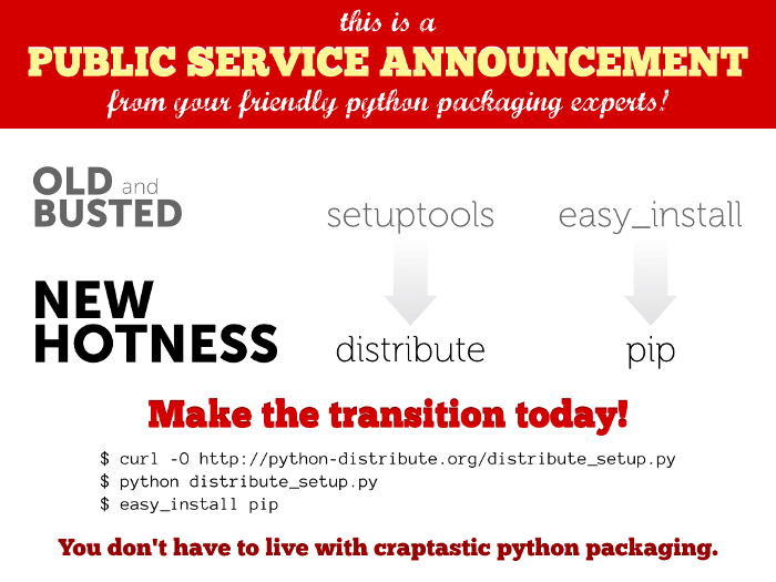
This text is a literal copy take from Martijn Faassen blog where he
describes the current (October 2010) state of packaging/distributing
Python software.
The reason I (Markus Gattol) include it here in full length again is
that I find it utterly important for anyone to understand the pig
picture about why things are the way the are today and what happened
during the last ten or so years so that we finally ended up with a
pretty amazing toolchain and infrastructure in order to develop,
package, distribute and share Python software.
Introduction
Earlier this year I (read Martijn Faassen) was at PyCon in the US. I
had an interesting experience there: people were talking about the
problem of packaging and distributing Python libraries. People had the
impression that this was an urgent problem that had not been solved
yet. I detected a vibe asking for the Python core developers to please
come and solve our packaging problems for us.
I felt like I had stepped into a parallel universe. I have been using
powerful tools to assemble applications from Python packages
automatically for years now. Last summer at EuroPython, when this
discussion came up again, I maintained that packaging and distributing
Python libraries is a solved problem. I put the point strongly, to
make people think. I fully agree that the current solutions are
imperfect and that they can be improved in many ways. But I also
maintain that the current solutions are indeed solutions.
There is now a lot of packaging infrastructure in the Python
community, a lot of technology, and a lot of experience. I think that
for a lot of Python developers the historical background behind all
this is missing. I will try to provide one here. It is important to
realize that progress has been made, step by step, for more than a
decade now, and we have a fine infrastructure today.
I have named some important contributors to the Python packaging
story, but undoubtedly I have also not mentioned a lot of other
important names. My apologies in advance to those I missed.
The dawn of Python packaging
The Python world has been talking about solutions for packaging and
distributing Python libraries for a very long time. I remember when I
was new in the Python world about a decade ago, in the late 90s, it
was considered important and urgent that the Python community
implement something like Perl's CPAN. I am sure too that this debate
had started long before I started paying attention.
I have never used CPAN, but over the years I have seen it held up by
many as something that seriously contributes to the power of the Perl
language. With CPAN, I understand, you can search and browse Perl
packages and you can install them from the net.
So, lots of people were talking about a Python equivalent to CPAN with
some urgency. At the same time, the Python world did not seem to move
very quickly on this front...
Distutils
The Distutils SIG (special interest group) was started in late 1998.
Greg Ward in the context of this discussion group started to create
Distutils about this time. Distutils allows you to structure your
Python project so that it has a setup.py. Through this setup.py you
can issue a variety of commands, such as creating a tarball out of
your project, or installing your project. Distutils importantly also
has infrastructure to help compiling C extensions for your Python
package. Distutils was added to the Python standard library in Python
1.6, released in 2000.
Metadata
We now had a way to distribute and install Python packages, if we did
the distribution ourselves. We did not have a centralized index (or
catalog) of packages yet, however. To work on this, the Catalog SIG
was started in the year
2000.
The first step was to standardize the metadata that could be cataloged
by any index of Python packages. Andrew Kuchling drove the effort on
this, culminating in PEP 241 in 2001, later updated by PEP 314.
Distutils was modified so it could work with this standardized
metadata.
PyPI
In late 2002, Richard Jones started work on the PyPI (Python Package
Index) — PyPI was initially known as the Cheeseshop. The first work
on an implementation started, and PEP 301 that describes PyPI was also
created then. Distutils was extended so the metadata and packages
themselves could be uploaded to this package index. By 2003, the
Python package index was up and running.
The Python world now had a way to upload packages and metadata
(actually known as distributions) to a central index. If we then
manually downloaded a package we could install it using setup.py
thanks to Distutils.
Setuptools
Phillip Eby started work on Setuptools in 2004. Setuptools is a whole
range of extensions to Distutils such as from a binary installation
format (eggs), an automatic package installation tool, and the
definition and declaration of scripts for installation. Work continued
throughout 2005 and 2006, and feature after feature was added to
support a whole range of advanced usage scenarios.
By 2005, you could install packages automatically into your Python
interpreter using EasyInstall. Dependencies would be automatically
pulled in. If packages contained C code it would pull in the binary
egg, or if not available, it would compile one automatically.
The sheer amount of features that Setuptools brings to the table must
be stressed: namespace packages, optional dependencies, automatic
manifest building by inspecting version control systems, web scraping
to find packages in unusual places, recognition of complex version
numbering schemes, and so on, and so on. Some of these features
perhaps seem esoteric to many, but complex projects use many of them.
The Problems of Shared Packages
The problem remained that all these packages were installed into your
Python interpreter. This is icky. People's site-packages directories
became a mess of packages. You also need root access to EasyInstall a
package into your system Python. Sharing all packages in a direcory in
general, even locally, is not always a good idea: one version of a
library needed by one application might break another one. Solutions
for this emerged in 2006.
Virtualenv
Ian Bicking drove one line of solutions: virtual-python, which evolved
into workingenv, which evolved into virtualenv in 2007. The concept
behind this approach is to allow the developer to create as many fully
working Python environments as they like from a central system
installation of Python. When the developer activates the virtualenv,
EasyInstall respectively its successor PIP will install all packages
into its the virtualenv's site-packages directory. This allows you to
create a virtualenv per project and thus isolate each project from
each other.
Buildout
In 2006 as well, Jim Fulton created Buildout, building on Setuptools
and EasyInstall. Buildout can create an isolated project environment
like virtualenv does, but is more ambitious: the goal is to create a
system for repeatable installations of potentially very complex
projects. Instead of writing an INSTALL.txt that tells others who to
install the prerequisites for a package (Python or not), with Buildout
these prerequisites can be installed automatically.
The brilliance of Buildout is that it is easily extensible with new
installation recipes. These recipes themselves are also installed
automatically from PyPI. This has spawned a whole ecosystem of
Buildout recipes that can do a whole range of things, from generating
documentation to installing MySQL.
Since Buildout came out of the Zope world, Buildout for a long time
was seen as something only Zope developers would use, but the
technology is not Zope-specific at all, and more and more developers
are picking up on it.
In 2008, Ian Bicking created an alternative for EasyInstall called
PIP, also building on Setuptools. Less ambitious than buildout, it
aimed to fix some of the shortcomings of EasyInstall. I have not used
it myself yet, so I will leave it to others to go into details.
Setuptools and the Standard Library
The many improvements that Setuptools brought to the Python packaging
story had not made it into the Python Standard Library, where
Distutils was stagnating. Attempts had been made to bring Setuptools
into the standard library at some point during its development, but
for one reason or another these efforts had foundered.
Setuptools probably got where it is so quickly because it worked
around often very slow process of adopting something into the standard
library, but that approach also helped confuse the situation for
Python developers.
Last year Tarek Ziade started looking into the topic of bringing
improvements into Distutils. There was a discussion just before PyCon
2009 about this topic between various Python developers as well, which
probably explains why the topic was in the air. I understood that some
decisions were made:
- Let the people with extensive packaging experience (such as Tarek)
drive this process.
- Free the metadata from Distutils and Setuptools so that other
packaging tools can make use of it more easily.
Distribute
By 2008, Setuptools had become a vital part of the Python development
infrastructure. Unfortunately the Setuptools development process has
some flaws. It is very centered around Phillip Eby. While he had been
extremely active before, by that time he was spending a lot less
energy on it. Because of the importance of the technology to the wider
community, various developers had started contributing improvements
and fixes, but these were piling up.
This year, after some period of trying to open up the Setuptools
project itself, some of these developers led by Tarek Ziade decided to
fork Setuptools. The fork is named Distribute. The aim is to develop
the technology with a larger community of developers. One of the first
big improvements of the Distribute project is Python 3 support.
Quite understandably this fork led to some friction between Tarek,
Phillip and others. I trust that this friction will resolve itself and
that the developers involved will continue to work with each other, as
all have something valuable contribute.
Packaging
From Setuptools to Distribute to distutils2 to packaging. Starting
with Python 3.3 packaging will replace distutils and become the
standard for packaging/distributing/installing.
Operating System Packaging
One point that always comes up in discussions about Python packaging
tools is operating system packaging. In particular Linux distributions
have developed extremely powerful ways to distribute and install
complex libraries and application, manage versions and dependencies
and so on.
Naturally when the topic of Python packaging comes up, people think
about operating system packaging solutions like this. Let me start off
that I fully agree that Python packaging solutions can learn a lot
from operating system packaging solutions.
Why don't we just use a solution like that directly, though? Why is a
Python specific packaging solution necessary at all?
There are a number of answers to this. One is that operating packaging
solutions are not universal: if we decided to use Debian's system,
what would we do on Windows?
The most important answer however is that there are two related but
also very different use cases for packaging:
- system administration: deploying and administrating existing software.
- development: combining software to develop new software.
The Python packaging systems described primarily tries to solve the
development use case: I am a Python developer, and I am developing
multiple projects at the same time, perhaps in multiple versions, that
have different dependencies. I need to reuse packages created by other
developers, so I need an easy way to depend on such packages. These
packages are sometimes in a rather early state of development, or
perhaps I am even creating a new one. If I want to improve such a
package I depend on, I need an easy way to start hacking on it.
Operating system packaging solutions as I have seen them used are ill
suited for the development use case. They are aimed at creating a
single consistent installation that is easy to upgrade with an eye on
security. Backwards compatibility is important. Packages tend to be
relatively mature.
For all I know it might indeed be possible to use an operating system
packaging tool as a good development packaging tool. But I have heard
very little about such practices. Please enlighten me if you have.
It is also important to note that the Python world is not as good as
it should be at supporting operating system packaging solutions. The
freeing up of package metadata from the confines of the setup.py file
into a more independently reusable format as was decided at PyCon
should help here.
Conclusions
We are now in a time of consolidation and opening up. Many of the
solutions pioneered by Setuptools are going to be polished to go into
the Python Standard Library. At the same time, the community
surrounding these technologies is opening up. By making metadata used
by Distutils and Setuptools more easily available to other systems,
new tools can also more easily be created.
The Python packaging story had many contributors over the years. We
now have a powerful infrastructure. Do we have an equivalent to CPAN?
I do not know enough about CPAN to be sure. But what we have is
certainly useful and valuable. In my parallel universe, I use advanced
Python packaging tools every day, and I recommend all Python
programmers to look into this technology if they have not already.
Join me in my parallel universe!
Update: I just found out there was a huge thread on python-dev about
this in the last few days which focused around the question whether we
have the equivalent of CPAN now. One of them funny coincidences...
History Continues
At PyCon 2010 the decision was made to basically exchange distutils
with distutils2 where distutils2 is a fork of Distribute. Setuptools,
distutils and Distribute are going to die (read phased out). pip will
stay and once distutils is replaced by distutils2, it will work with
it as it does now (October 2010) with Distribute. Take a look at this
picture:
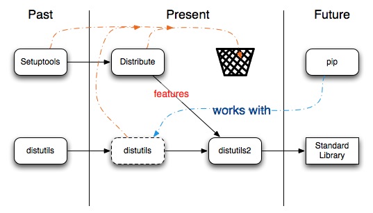
- The distutils module is currently part of the standard library and
will be until Python 3.3 — it will be discontinued in Python 3.3
in favor of
distutils2 which will be backwards compatible down to
Python 2.4.
- Update: In May 2011 packaging was announced — it is
distutils2
renamed to packaging and is now part of the standard library in
Python 3.
Glossary
WRITEME
Examples
Just provide the below links and then show a bunch of examples for
each step i.e. package, distribute, install; thereby using the tools
(pip, distribute, etc.) listed below
WRITEME
Tools, Utilities
This section provides information on what tools I use on a daily basis
when it comes to developing/deploying/administer/test/etc. Python
software.
pythonrc
When using the interactive interpreter it is frequently handy to have
some code executed every time the interpreter is started e.g. to load
some module or to set some environment variable etc.
We can do this by setting the environment variable PYTHONSTARTUP to
the name of a file containing our start-up code (~/.pythonrc for
example) e.g. we can put export
PYTHONSTARTUP=$HOME/.pythonrc inside ~/.bashrc. All the startup
file contains is Python code that gets executed at startup of the
interpreter. Below is the current version of my ~/.pythonrc:
sa@wks:~$ cat .pythonrc
#!/usr/bin/env python
"""Initialization file for the Python interpreter.
This is the initialization file for the Python interpreter used in
interactive sessions. Some general pointers:
- /ws/python.html#pythonrc
- /ws/python.html#bpython
"""
__author__ = "Markus Gattol"
__author_email__ = "[email protected]"
__copyright__ = "Copyright (C) 2012 Free Software Foundation, Inc."
__development_status__ = "Production/Stable"
__license__ = "Simplified BSD License"
__url__ = "/ws/python.html"
__version__ = "1.0"
#_ main
#_. imports
import sys
import os
import pprint
#_. import saved bpython sessions if available
try:
from startup import * # do not do that in real code
print("Successful import from startup.py.")
except ImportError:
print("No startup file available.")
#_. colored prompt and autocompletion
if os.getenv('TERM') in ('xterm', 'vt100', 'rxvt', 'Eterm', 'putty'):
try:
import readline
except ImportError:
print("Module readline not available.")
sys.ps1 = '\033[01;33m>>> \033[0m'
sys.ps2 = '\033[01;33m... \033[0m'
else:
import rlcompleter
readline.parse_and_bind("tab: complete")
sys.ps1 = '\001\033[01;33m\002>>> \001\033[0m\002'
sys.ps2 = '\001\033[01;33m\002... \001\033[0m\002'
#_. fast way to show what is on sys.path
try:
def show_sys_path():
"""Prints a pretty version of everything on sys.path.
We do this because having one output per line is easier to
read compared to having several outputs on a single line.
"""
pprint.pprint(sys.path)
# show automatically when starting the interactive interpreter
print("sys.path currently holds:")
show_sys_path()
except ImportError:
print("Module pprint not available.")
#_. shadow sys.display hook with pprint variant
def my_displayhook(value):
"""Overriding the built-in version with our own.
We do this because having one output per line is easier to read
compared to having several outputs on a single line.
"""
if value is not None:
try:
import __builtin__
__builtin__._ = value
except ImportError: # not Python 2 but Python 3
import builtins
builtins._ = value
pprint.pprint(value)
sys.displayhook = my_displayhook
#_. do for bpython what shell_plus from django-extensions does for ipython
try:
from django.core.management import setup_environ
from django.conf import settings
try:
import settings
setup_environ(settings)
print("Sucessfully imported Django settings.")
except ImportError: # non-standard place for config
import config.settings
setup_environ(config.settings)
print("Sucessfully imported Django settings.")
try:
print("Attempting to import Django models:")
from django.db.models.loading import get_models, get_apps
for app in get_apps():
app_models = get_models(app)
if not app_models:
continue
model_labels = ", ".join([model.__name__ for model in app_models])
try:
exec("from %s import *" % app.__name__)
print(" From '%s' load: %s" % (app.__name__.split('.')[-2],
model_labels))
except Exception:
print(" Not imported for '%s'" % app.__name__.split('.')[-2])
except ImportError:
pass
except ImportError:
pass
#_ emacs local variables
# Local Variables:
# mode: python
# allout-layout: (0 : 0)
# End:
All right, now let us check if we wrote a good module or not:
sa@wks:~$ pep8 .pythonrc # all good for pep8 (no output)
sa@wks:~$ pylint --disable=F0401,W0703,W0122,W0611,C0301 .pythonrc # all good for pylint as well
sa@wks:~$ echo; pylint --help-msg=F0401,W0703,W0122,W0611,C0301 # closer look of what we ignored
:F0401: *Unable to import %r*
Used when pylint has been unable to import a module. This message
belongs to the imports checker.
:W0703: *Catch "Exception"*
Used when an except catches Exception instances. This message
belongs to the exceptions checker.
:W0122: *Use of the exec statement*
Used when you use the "exec" statement, to discourage its usage.
That doesn't mean you can not use it ! This message belongs to the
basic checker.
:W0611: *Unused import %s*
Used when an imported module or variable is not used. This message
belongs to the variables checker.
:C0301: *Line too long (%s/%s)*
Used when a line is longer than a given number of characters. This
message belongs to the format checker.
sa@wks:~$
pep8 tells us nothing (no output), meaning everything is fine. pylint
however would moan about a few things but then we decide that we
ignore those because we know about it and it is actually fine to
ignore those pylint tests in case of ~/.pythonrc as it stands.
BPython
Is there a better Python Shell/Interpreter? Yes, yes, there is! There
is iPython and then there is bpython which I have come to love. It is
packaged with Debian
sa@wks:~$ dpkg -l bpython | grep ii
ii bpython 0.9.7.1-1 fancy interface to the Python interpreter - Curses frontend
sa@wks:~$
There is also http://bpaste.net, a pastebin site. This for itself is
no big deal. The fact that bpython can ship off its contents (what we
typed) at the press of a button, right into bpaste.net, however is —
I often use it to sketch things in a live interpreter session and then
quickly show it to folks while we talk on IRC, maybe during debugging
some code and stuff like that.
There are a lot more goodies at our disposal like for example
Django support. Most of it can be configured in ~/.bpython/config:
sa@wks:~$ cat .bpython/config | grep -v \# | grep .
[general]
auto_display_list = True
syntax = True
arg_spec = True
hist_file = ~/.pythonhist
hist_len = 5000
tab_length = 4
color_scheme = suno
[keyboard]
pastebin = F8
save = C-s
And then there is of course a custom theme we might use
sa@wks:~$ cat .bpython/suno.theme | grep -v \# | grep .
[syntax]
keyword = y
name = W
comment = w
string = M
error = r
number = G
operator = Y
punctuation = y
token = C
[interface]
background = d
output = w
main = w
prompt = w
prompt_more = w
sa@wks:~$
The coolest thing about bpython is probably autocompletion, inline
syntax highlighting, the fact that is shows us the expected parameter
list as we type and last but not least, the possibility to rewind what
we typed not just graphically but also internally i.e. the results of
each such expression we typed. Below is a screenshot showing a few of
the just mentioned things:
Multiple Python Versions
Currently (March 2011) we can run bpython with those Python versions:
2.4, 2.5, 2.6, 2.7 and 3. The default version is the one our Debian
system links to:
sa@wks:~$ type ll; ll $(which python)
ll is aliased to `ls -lh -I "*\.pyc"'
lrwxrwxrwx 1 root root 9 Jan 17 07:53 /usr/bin/python -> python2.6
sa@wks:~$
However, we can use others as well simply by creating an alias in our
~/.bashrc:
sa@wks:~$ grep ', bpython' -A9 .bashrc
###_ , bpython
# use whatever python is default plus consider environment
alias bp='/usr/bin/env bpython'
# try to force python2.6; does not consider environment
alias bp2='$(which python2.6) -m bpython.cli'
# try to force python2.6; does not consider environment
alias bp3='$(which python3) -m bpython.cli'
sa@wks:~$
The added benefit of /usr/bin/env is that it takes the current
environment into account e.g. whether or not we are currently using a
virtual environment or not. In case we are using a virtual
environment, and have installed bpython into it, this version of
bpython will be used when using the bp alias.
bpython and Python 3
Currently (March 2011) there is no bpython Debian package for Python
3, only for Python 2. That is no problem however, we can install from
source:
- we use
hg clone https://bitbucket.org/bobf/bpython to get the
source code
- next we install (as
root) bpython for Python 3 using python3
setup.py install from within the just cloned ../bpython directory
- finally we add the aliases as shown. Now issuing
bp will start
bpython with Python 3, if we need/want to run bpython with Python
2, bp2 will do the trick. And in general, as mentioned, the bp
alias will also take into account a virtual environment, launching
bpython on top of whatever Python is installed. Nine out of ten
times I simply type bp because it is exactly what I need.
bpython and Virtualenv
If we want to use bpython from within a virtual environment, then we
need to do three things:
install bpython into virtual environment
One, we install bpython into each virtual environment using pip
install bpython.
modify .pythonrc
If a ~/.pythonrc is used then we add a pound bang line at the top
sa@wks:~$ head -n1 .pythonrc
#!/usr/bin/env python
sa@wks:~$
What happens now is that /usr/bin/env (see man 1 env) looks at our
PATH environment variable and then provides us with the correct Python
interpreter and runtime environment i.e. we either get the one from a
virtual environment or the one from the global Python context/space,
all depending on whether or not some virtual environment is active or
not.
bpython Environment Awareness
Last but not least, we start bpython so that the current environment
is taken into account. We can use a simple shell alias for that.
bpython and Django
Usually, being at the root of a Django project, which we created using
django-admin startproject, we could issue python manage.py shell which
runs iPython if available:
sa@wks:~/0/django/myproject$ python manage.py help shell | grep Runs
Runs a Python interactive interpreter. Tries to use IPython, if it's available.
sa@wks:~/0/django/myproject$
If however we want python manage.py shell to use bpython instead, here
is what we can do: We start with using PYTHONSTARTUP i.e. we put
export PYTHONSTARTUP=$HOME/.pythonrc into our ~/.bashrc
file. Next, we put Python into ~/.pythonrc to make python manage.py
shell use bpython instead of iPython.
The rationale behind PYTHONSTARTUP is simple: When we use Python
interactively, it is frequently handy to have some standard commands
executed every time the interpreter is started. We can do this by
setting the environment variable PYTHONSTARTUP to the name of a file
containing our start-up commands (~/.pythonrc for example). This is no
Python speciallity as it is the same as ~/.profile, ~/.bashrc and
friends are for any Unix shell out there...
Note that whatever file PYTHONSTARTUP points to, it is only read in
interactive sessions, not when Python reads commands from a script,
and not when /dev/tty is given as the explicit source of commands
(which otherwise behaves like an interactive session). It is executed
in the same namespace where interactive commands are executed, so that
objects that it defines or imports can be used without qualification
in the interactive session.
Furthermore, we can also change the prompts sys.ps1 (>>>) and sys.ps2
(...) in this file — those are the primary respectively secondary
prompts of the interpreter. They are only defined if the interpreter is
in interactive mode.
Now that we have PYTHONSTARTUP in place and use it to point to
~/.pythonrc, we can use it to do all kinds of setup work like for
example setup the Django environment i.e. what we do here manually is
the same what python manage.py shell otherwises does for us
automatically. Below is the source code taken from ~/.pythonrc to get
this behavior with bpython:
[skipping a lot of lines...]
#_. do for bpython what shell_plus from django-extensions does for ipython
try:
from django.core.management import setup_environ
from django.conf import settings
try:
import settings
setup_environ(settings)
print("Sucessfully imported Django settings.")
except ImportError:
import config.settings
setup_environ(config.settings)
print("Sucessfully imported Django settings.")
try:
print("Attempting to import Django models:")
from django.db.models.loading import get_models, get_apps
for app in get_apps():
app_models = get_models(app)
if not app_models:
continue
model_labels = ", ".join([model.__name__ for model in app_models])
try:
exec("from %s import *" % app.__name__)
print(" From '%s' load: %s" % (app.__name__.split('.')[-2],
model_labels))
except Exception:
print(" Not imported for '%s'" % app.__name__.split('.')[-2])
except ImportError:
pass
except ImportError:
pass
[skipping a lot of lines...]
With this in place bpython (or even just the ordinary Python
interpreter) imports the Django environment for us. Let us now have a
look at what it looks/feels like when we issue our bp alias from
within an activated virtual environment which already has a Django
project installed:
(aa) sa@wks:~/0/python/projects/aa$ bp
No startup file available.
sys.path currently holds:
['',
'/home/sa/0/1/aa/bin',
'/home/sa/0/1/aa/lib/python2.6/site-packages/distribute-0.6.10-py2.6.egg',
'/home/sa/0/1/aa/lib/python2.6/site-packages/pip-0.7.2-py2.6.egg',
'/home/sa/.pip/source/django-authorizenet',
'/home/sa/.pip/source/django-dbindexer',
[skipping a lot of lines...]
'/home/sa/0/python/projects/aa',
'/home/sa/0/1/aa',
'/home/sa/0/python/projects/aa/apps']
Sucessfully imported Django settings.
Attempting to import Django models:
From 'auth' load: Permission, Group, User, Message
From 'contenttypes' load: ContentType
From 'sessions' load: Session
From 'sites' load: Site
From 'polls' load: Poll, Choice
From 'admin' load: LogEntry
From 'socialregistration' load: FacebookProfile, TwitterProfile, OpenIDProfile, OpenIDStore, OpenIDNonce
From 'featureflipper' load: Feature
From 'reversion' load: Revision, Version
From 'djcelery' load: TaskMeta, TaskSetMeta, IntervalSchedule, CrontabSchedule, PeriodicTasks, PeriodicTask, WorkerState, TaskState
>>>
We started bpython from within an activated virtual environment and it
gave us all kinds of goodies right out of the box — that is because
~/.pythonrc has been used (compare the output from above with the code
from ~/.pythonrc). What else is there? Let us have a further look:
>>> settings.INSTALLED_APPS
['django_mongodb_engine',
'django.contrib.auth',
'django.contrib.contenttypes',
'django.contrib.sessions',
'django.contrib.sites',
'django.contrib.messages',
'polls',
'django.contrib.admin',
[skipping a lot of lines...]
'dbindexer']
>>> sys.displayhook
<function my_displayhook at 0x1c10380>
>>> len(dir())
104
>>> exit()
~/.pythonrc takes care of importing all the settings for our Django
project so we can do things like list the contents of INSTALLED_APPS
right away. We can also see that we get nice listings because we
shadow sys.displayhook with our own my_displayhook function. Another
indicator that our ~/.pythonrc is doing a great job is when we look at
dir() which, without arguments, returns a list of names in the current
local scope. With a vanilla Python environment those are usually just
around 4, rather than 104.
(aa) sa@wks:~/0/python/projects/aa$ cat apps/polls/models.py
import datetime
from django.db import models
class Poll(models.Model): # real code would have docstrings
question = models.CharField(max_length=200)
pub_date = models.DateTimeField('date published')
def __unicode__(self):
return self.question
def was_published_today(self):
return self.pub_date.date() == datetime.date.today()
was_published_today.short_description = 'Published today?'
class Choice(models.Model):
poll = models.ForeignKey(Poll)
choice = models.CharField(max_length=200)
votes = models.IntegerField()
def __unicode__(self):
return self.choice
(aa) sa@wks:~/0/python/projects/aa$
Within our Django project we have created a Django application called
polls. We can see that polls was one of the already imported Django
applications which has the Poll and Choice models — we do not need to
do the import ourselves anymore but can start using them right away:
(aa) sa@wks:~/0/python/projects/aa$ bp
No startup file available.
sys.path currently holds:
['',
'/home/sa/0/1/aa/bin',
'/home/sa/0/1/aa/lib/python2.6/site-packages/distribute-0.6.10-py2.6.egg',
[skipping a lot of lines...]
From 'reversion' load: Revision, Version
From 'djcelery' load: TaskMeta, TaskSetMeta, IntervalSchedule, CrontabSchedule, PeriodicTasks, PeriodicTask, WorkerState, TaskState
>>> Poll.objects.all()
[]
>>> p = Poll(question="What's up?", pub_date=datetime.now())
>>> p.save()
>>> p.id
u'4d63beba4ed6db0e36000000'
>>> type(p.id)
<type 'unicode'>
>>> p.question
"What's up?"
>>> p.pub_date
datetime.datetime(2011, 2, 22, 7, 46, 47, 917063)
>>> p.was_published_today()
True
>>>
Nothing unusual there except for p.id which actually returns a unicode
string rather than an integer — that is because I am using MongoDB
rather than some RDBMS (Relational Database Management System) such as
MySQL or SQLite.
Startup File
Last but not least, we can use bpython's ability to save the current
session to a file. This file is then used to load our former session
into bpython again, effectively allowing us to resume our work where
we left off before. The way this is accomplished is also by using
~/.pythonrc:
[skipping a lot of lines...]
#_. import saved bpython sessions if available
try:
from startup import * # do not do that in real code
print("Successful import from startup.py.")
except ImportError:
print("No startup file available.")
[skipping a lot of lines...]
We can then use the C+s keys and when prompted for the filename to
save our session, we use startup.py:
>>> print("funky donkey at work")
funky donkey at work
>>> foo = range(4)
>>> foo
[0, 1, 2, 3]
>>>
[ here I used C+s to save the current session to startup.py... ]
>>> exit()
(aa) sa@wks:~/0/python/projects/aa$ cat startup.py
print("funky donkey at work")
# OUT: funky donkey at work
foo = range(4)
foo
# OUT: [0, 1, 2, 3]
(aa) sa@wks:~/0/python/projects/aa$ bp
funky donkey at work
Successful import from startup.py.
sys.path currently holds:
['',
'/home/sa/0/1/aa/bin',
'/home/sa/0/1/aa/lib/python2.6/site-packages/distribute-0.6.10-py2.6.egg',
[skipping a lot of lines...]
From 'reversion' load: Revision, Version
From 'djcelery' load: TaskMeta, TaskSetMeta, IntervalSchedule, CrontabSchedule, PeriodicTasks, PeriodicTask, WorkerState, TaskState
>>> foo
[0, 1, 2, 3]
>>>
Note how it now printed funky donkey at work rather than No startup
file available. We also have foo available because, as we can see, it
got replayed from startup.py when we started bpython again after we
used to save to startup.py in the last session.
Virtualenv, Virtualenvwrapper
This one is all about gaining freedom — the kind of freedom that
allows us to be creative, have fun and get things done quickly and in
a straight forward and simple manner. So, what is it that virtualenv
does in a nutshell?
By using virtualenv and possibly virtualenvwrapper and/or
virtualenv-commands on top of it, we can create sanboxes also known as
virtual environments. What this gives us is the benefit of isolated
environments i.e. we can work without risking to mess up the rest of
our system by mistake.
Virtual environments are isolated by default but we can also have
symlinks leaving it and going into our global Python context/space —
the installation-dependent default path and the global Python
interpreter living at /usr/bin/python on Debian. All we need to do is
use the --system-site-packages switch to virtualenv.
Note that this behavior changed in October 2011. Before that virtual
environments were not isolated by default but were integrated with the
global Python context/space by default and one had to use the
--no-site-packages switch to get an isolated virtual environment.
As said, nowadays the default behavior is that those sandboxes are
isolated from the rest of the system (no outgoing symlinks), meaning
that by using a virtual environment, we can try out software, alter
software, add/remove things, etc. — all without any danger of
accidentally doing something stupid to our global Python
context/space.
This makes virtual environments the perfect tool for testbeds, staging
environments, versioned deployments... virtualenv is basically a
Python symmetric link utility for cloning an existing Python
installation or creating an entirely separated one so that we can
easily install/uninstall/develop Python software at a different
location than the standard one.
Installing and setting up Virtualenv
Installing virtualenv is easy. Debian provides a package for it
sa@wks:~$ type dpl; dpl *virtualenv | grep ii
dpl is aliased to `dpkg -l'
ii python-virtualenv 1.6-4 Python virtual environment creator
sa@wks:~$ virtualenv --version
1.6.4
sa@wks:~$ virtualenv --help
Usage: virtualenv [OPTIONS] DEST_DIR
Options:
--version show program's version number and exit
-h, --help show this help message and exit
-v, --verbose Increase verbosity
-q, --quiet Decrease verbosity
-p PYTHON_EXE, --python=PYTHON_EXE
The Python interpreter to use, e.g.,
--python=python2.5 will use the python2.5 interpreter
to create the new environment. The default is the
interpreter that virtualenv was installed with
(/usr/bin/python)
--clear Clear out the non-root install and start from scratch
--system-site-packages
Give access to the global site-packages dir to the
virtual environment
--unzip-setuptools Unzip Setuptools or Distribute when installing it
--relocatable Make an EXISTING virtualenv environment relocatable.
This fixes up scripts and makes all .pth files
relative
--distribute Use Distribute instead of Setuptools. Set environ
variable VIRTUALENV_USE_DISTRIBUTE to make it the
default
--extra-search-dir=SEARCH_DIRS
Directory to look for setuptools/distribute/pip
distributions in. You can add any number of additional
--extra-search-dir paths.
--never-download Never download anything from the network. Instead,
virtualenv will fail if local distributions of
setuptools/distribute/pip are not present.
--prompt==PROMPT Provides an alternative prompt prefix for this
environment
sa@wks:~$
Of course, one could also use easy_install virtualenv or even better,
pip install virtualenv but then it is probably best to use Debian's
package for the global Python context/space (the opposite of a virtual
environment context/space created using virtualenv) right away — I
tend to sometimes replicate systems (e.g. when I swap the HDD in my
subnotebook for a SSD (Solid State Drive)) in which case it is easy to
automatically replicate the set of installed Debian packages so...
Using Virtualenv
Basically, what we need to know is how to create a new virtual
environment (line 1), enter and activate it (lines 31 and 32), carry
out some commands (e.g. line 33, looking what Python interpreter is
currently active) and last but not least, switch back from the virtual
environment into the global Python context/space (line 35) and yet
again, look up the currently active Python interpreter (lines 36 and
37):
1 sa@wks:~/0/1$ virtualenv my_test_virt_env
2 New python executable in my_test_virt_env/bin/python
3 Installing distribute..................done.
4 Installing pip.....................done.
5 sa@wks:~/0/1$ type td; td my_test_virt_env/
6 td is aliased to `tree --charset ascii -d -I \.git*\|*\.\~*\|*\.pyc'
7 my_test_virt_env/
8 |-- bin
9 |-- include
10 | `-- python2.7 -> /usr/include/python2.7
11 |-- lib
12 | `-- python2.7
13 | |-- config -> /usr/lib/python2.7/config
14 | |-- distutils
15 | |-- encodings -> /usr/lib/python2.7/encodings
16 | |-- lib-dynload -> /usr/lib/python2.7/lib-dynload
17 | `-- site-packages
18 | |-- distribute-0.6.19-py2.7.egg
19 | | |-- EGG-INFO
20 | | `-- setuptools
21 | | |-- command
22 | | `-- tests
23 | `-- pip-1.0.2-py2.7.egg
24 | |-- EGG-INFO
25 | `-- pip
26 | |-- commands
27 | `-- vcs
28 `-- local -> /home/sa/0/1/my_test_virt_env
29
30 21 directories
31 sa@wks:~/0/1$ cd my_test_virt_env/
32 sa@wks:~/0/1/my_test_virt_env$ source bin/activate
33 (my_test_virt_env)sa@wks:~/0/1/my_test_virt_env$ which python
34 /home/sa/0/1/my_test_virt_env/bin/python
35 (my_test_virt_env)sa@wks:~/0/1/my_test_virt_env$ deactivate
36 sa@wks:~/0/1/my_test_virt_env$ which python
37 /usr/bin/python
38 sa@wks:~/0/1/my_test_virt_env$ cd
The whole point of using virtualenv can be best seen from lines 34 and
37 — first we use a virtual environment and therefore our Python
interpreter lives at /home/sa/0/1/my_test_virt_env/bin/python but then
we are back in the global Python context/space where we would use
/usr/bin/python. By the way, td from line 5 is just an alias in my
~/.bashrc.
Virtualenvwrapper
Virtualenvwrapper is a set of extensions to virtualenv. The extensions
include wrappers for creating and deleting virtual environments and
otherwise managing our development workflow, making it easier to work
on more than one project at a time without introducing conflicts in
their dependencies.
Installing and activating virtualenvwrapper is easy — one might
either use pip install virtualenvwrapper or, in my opinion even
better, go straight for the aptitude install virtualenvwrapper option
which works out of the box in case we also have bash-completion
installed and enabled it in /etc/bash.bashrc (see
/usr/share/doc/virtualenvwrapper/README.Debian for more information).
Next we are going to address our ~/.bashrc file:
37 sa@wks:~$ grep -A4 ', virtualenvwrapper' .bashrc
38 ###_ , virtualenvwrapper
39 export WORKON_HOME=$HOME/0/1
40 alias cdveroots='cd $WORKON_HOME'
41
42
43 sa@wks:~$ source .bashrc; echo $WORKON_HOME
44 /home/sa/0/1
The important part here is with line 39 where we tell
virtualenvwrapper where our virtual environments are going to live on
the filesystem.
With line 40 we also add an alias which is going to save us a lot of
time down the road since it always beams us back into $WORKON_HOME no
matter where we are on the filesystem — in my case that is
/home/sa/0/1 as can be seen from line 44.
Excellent! We are done installing and setting up virtualenv and
virtualenvwrapper. More information can be found here, here and here.
Usage Examples - Commands
We have a bunch of commands that come with the virtualenvwrapper
package as can be seen below. This is a snapshot of the current
situation (September 2011). Of course, there might be
additions/changes in the future.
sa@wks:~$ egrep '^[[:alpha:]]+.*\(\) {' /etc/bash_completion.d/virtualenvwrapper | grep -v _ | cut -f1 -d ' '
mkvirtualenv
rmvirtualenv
lsvirtualenv
showvirtualenv
workon
add2virtualenv
cdsitepackages
cdvirtualenv
lssitepackages
toggleglobalsitepackages
cpvirtualenv
sa@wks:~$
Next I am going to provide a few examples about how to use some of the
commands so folks can see how things work right away:
45 sa@wks:~$ workon
46 my_test_virt_env
47 sa@wks:~$ workon my_test_virt_env
48 (my_test_virt_env)sa@wks:~$ cdvirtualenv
49 (my_test_virt_env)sa@wks:~/0/1/my_test_virt_env$ cdveroot
50 (my_test_virt_env)sa@wks:~/0/1$ ll
51 total 4.0K
52 drwxr-xr-x 5 sa sa 4.0K Sep 1 13:46 my_test_virt_env
53 (my_test_virt_env)sa@wks:~/0/1$ cd /tmp
54 (my_test_virt_env)sa@wks:/tmp$ cdvirtualenv
55 (my_test_virt_env)sa@wks:~/0/1/my_test_virt_env$ pwd
56 /home/sa/0/1/my_test_virt_env
57 (my_test_virt_env)sa@wks:~/0/1/my_test_virt_env$ echo $VIRTUALENVWRAPPER_HOOK_DIR
58 /home/sa/.virtualenvs
59 (my_test_virt_env)sa@wks:~/0/1/my_test_virt_env$ ll $VIRTUALENVWRAPPER_HOOK_DIR
60 total 44K
61 -rwxrwxr-x 1 sa sa 106 May 11 10:18 get_env_details
62 -rw-r--r-- 1 sa sa 3.7K Sep 1 14:15 hook.log
63 -rwxrwxr-x 1 sa sa 92 May 11 10:18 initialize
64 -rwxr-xr-x 1 sa sa 1.3K Sep 1 14:06 postactivate
65 -rwxrwxr-x 1 sa sa 71 May 11 10:18 postdeactivate
66 -rwxr-xr-x 1 sa sa 122 Sep 1 13:37 postmkvirtualenv
67 -rwxrwxr-x 1 sa sa 63 May 11 10:18 postrmvirtualenv
68 -rwxrwxr-x 1 sa sa 70 May 11 10:18 preactivate
69 -rwxrwxr-x 1 sa sa 72 May 11 10:18 predeactivate
70 -rwxrwxr-x 1 sa sa 94 May 11 10:18 premkvirtualenv
71 -rwxrwxr-x 1 sa sa 64 May 11 10:18 prermvirtualenv
72 (my_test_virt_env)sa@wks:~/0/1/my_test_virt_env$
The command reference list all commands available. My favorite is
probably workon and cdvirtualenv — the former is used to list/switch
amongst virtual environments and the later one to beam us right back
into the root of the currently activated virtual environment no matter
where we are on the filesystem. Gosh! I love it! About lines 61 to 71,
those are hooks which I will tell more about later.
73 (my_test_virt_env)sa@wks:~/0/1$ deactivate
74 sa@wks:~/0/1$ mkvirtualenv test
75 New python executable in test/bin/python
76 Installing distribute....................................................................................................................................................................................done.
77 virtualenvwrapper.user_scripts creating /home/sa/0/1/test/bin/predeactivate
78 virtualenvwrapper.user_scripts creating /home/sa/0/1/test/bin/postdeactivate
79 virtualenvwrapper.user_scripts creating /home/sa/0/1/test/bin/preactivate
80 virtualenvwrapper.user_scripts creating /home/sa/0/1/test/bin/postactivate
81 virtualenvwrapper.user_scripts creating /home/sa/0/1/test/bin/get_env_details
82 (test)sa@wks:~/0/1$ workon
83 my_test_virt_env
84 test
Line 73 shows how easy it is to create a new virtual environment using
mkvirtualenv. Note that command line arguments to virtualenvwrapper
are passed right through to virtualenv! Also note that by creating our
new virtual environment test using mkvirtualenv, we switched right to
it as can be seen in line 82.
We now have two virtual environments (lines 83 and 84) which can be
listed using workon without any argument.
85 (test)sa@wks:~/0/1$ workon my_test_virt_env
86 (my_test_virt_env)sa@wks:~/0/1$ cdvirtualenv
87 (my_test_virt_env)sa@wks:~/0/1/my_test_virt_env$ rmvirtualenv my_test_virt_env
88 ERROR: You cannot remove the active environment ('my_test_virt_env').
89 Either switch to another environment, or run 'deactivate'.
90 (my_test_virt_env)sa@wks:~/0/1/my_test_virt_env$ rmvirtualenv test
91 (my_test_virt_env)sa@wks:~/0/1/my_test_virt_env$ workon
92 my_test_virt_env
Lines 85 to 93 show a few things about deleting a virtual environment.
As we can see from lines 87 to 89, deleting/removing the currently
active virtual environment does not work — this is a safety switch
provided by virtualenvwrapper. As lines 90 to 92 show, our former
created virtual environment test has been removed — basically this is
the same as using rm -r /home/sa/0/1/test but then rmvirtualenv takes
care not to wipe out the currently active virtual environment.
93 (my_test_virt_env)sa@wks:~/0/1/my_test_virt_env$ cd
94 (my_test_virt_env)sa@wks:~$ cdvirtualenv bin
95 (my_test_virt_env)sa@wks:~/0/1/my_test_virt_env/bin$ pwd
96 /home/sa/0/1/my_test_virt_env/bin
97 (my_test_virt_env)sa@wks:~/0/1/my_test_virt_env/bin$
98 (my_test_virt_env)sa@wks:~/0/1/my_test_virt_env/bin$ cdsitepackages
99 (my_test_virt_env)sa@wks:~/0/1/my_test_virt_env/lib/python2.6/site-packages$ pwd
100 /home/sa/0/1/my_test_virt_env/lib/python2.6/site-packages
Since I am such a fan of cdvirtualenv, line 94 shows us more of its
magic — appending an argument such as bin does not beam us back into
the root of the currently active virtual environment but actually
moves us down one level into /home/sa/0/1/my_test_virt_env/bin. Gosh
the 2nd! ;-]
cdvirtualenv has a friend called cdsitepackages which is no less
amazing as it beams us right into the site-packages directory of our
currently activated virtual environment. Now listing its contents
would be a simple matter of using ls.
101 (my_test_virt_env)sa@wks:~/0/1/my_test_virt_env/lib/python2.6/site-packages$ cd
102 (my_test_virt_env)sa@wks:~$ lssitepackages
103 distribute-0.6.15-py2.6.egg easy-install.pth pip-1.0-py2.6.egg setuptools.pth
104 (my_test_virt_env)sa@wks:~$ lssitepackages -l
105 total 16
106 drwxr-xr-x 4 sa sa 4096 Sep 1 14:07 distribute-0.6.15-py2.6.egg
107 -rw-r--r-- 1 sa sa 235 Sep 1 13:46 easy-install.pth
108 drwxr-xr-x 4 sa sa 4096 Sep 1 14:07 pip-1.0-py2.6.egg
109 -rw-r--r-- 1 sa sa 30 Sep 1 14:07 setuptools.pth
110 (my_test_virt_env)sa@wks:~$ cd /tmp
However, what if we just wanted to know its contents without visiting
../site-packages/? Easy, we use lssitepackages as shown in lines 102
and 104 respectively. Line 102 lists all contents of
/home/sa/0/1/my_test_virt_env/lib/python2.6/site-packages even though
we are currently inside /home/sa. Also, again, note how the -l switch
gets passed through in line 104.
The last command we are going to take a look at is add2virtualenv. It
is used to link code into the currently active virtual environment.
Note that linking here does not determine a symmetrical link but
rather adding another path to Python's module search paths.
111 (my_test_virt_env)sa@wks:/tmp$ git clone git://github.com/pinax/pinax.git
112 Cloning into pinax...
113 remote: Counting objects: 40935, done.
114 remote: Compressing objects: 100% (13975/13975), done.
115 remote: Total 40935 (delta 23793), reused 39744 (delta 22788)
116 Receiving objects: 100% (40935/40935), 15.18 MiB | 969 KiB/s, done.
117 Resolving deltas: 100% (23793/23793), done.
118 (my_test_virt_env)sa@wks:/tmp$ cdvirtualenv
119 (my_test_virt_env)sa@wks:~/0/1/my_test_virt_env$ python
120 Python 2.6.7 (r267:88850, Aug 3 2011, 11:33:52)
121 [GCC 4.6.1] on linux2
122 Type "help", "copyright", "credits" or "license" for more information.
123 No startup.py file available.
124 sys.path currently holds:
125 ['',
126 '/home/sa/0/1/my_test_virt_env/lib/python2.6/site-packages/distribute-0.6.15-py2.6.egg',
127 '/home/sa/0/1/my_test_virt_env/lib/python2.6/site-packages/pip-1.0-py2.6.egg',
128 '/home/sa/0/1/my_test_virt_env/lib/python2.6',
129 '/home/sa/0/1/my_test_virt_env/lib/python2.6/plat-linux2',
130 '/home/sa/0/1/my_test_virt_env/lib/python2.6/lib-tk',
131 '/home/sa/0/1/my_test_virt_env/lib/python2.6/lib-old',
132 '/home/sa/0/1/my_test_virt_env/lib/python2.6/lib-dynload',
133 '/usr/lib/python2.6',
134 '/usr/lib/python2.6/plat-linux2',
135 '/usr/lib/python2.6/lib-tk',
136 '/home/sa/0/1/my_test_virt_env/lib/python2.6/site-packages']
137 >>>
138 (my_test_virt_env)sa@wks:~/0/1/my_test_virt_env$ cdsitepackages
139 (my_test_virt_env)sa@wks:~/0/1/my_test_virt_env/lib/python2.6/site-packages$ type pi; pi pth
140 pi is aliased to `ls -la | grep'
141 -rw-r--r-- 1 sa sa 235 Sep 1 13:46 easy-install.pth
142 -rw-r--r-- 1 sa sa 30 Sep 1 14:07 setuptools.pth
143 (my_test_virt_env)sa@wks:~/0/1/my_test_virt_env/lib/python2.6/site-packages$ add2virtualenv /tmp/pinax/
144 Warning: Converting "/tmp/pinax/" to "/tmp/pinax"
145 (my_test_virt_env)sa@wks:~/0/1/my_test_virt_env/lib/python2.6/site-packages$ pi pth
146 -rw-r--r-- 1 sa sa 235 Sep 1 13:46 easy-install.pth
147 -rw-r--r-- 1 sa sa 30 Sep 1 14:07 setuptools.pth
148 -rw-r--r-- 1 sa sa 11 Sep 1 14:41 virtualenv_path_extensions.pth
149 (my_test_virt_env)sa@wks:~/0/1/my_test_virt_env/lib/python2.6/site-packages$ cat virtualenv_path_extensions.pth
150 /tmp/pinax
151 (my_test_virt_env)sa@wks:~/0/1/my_test_virt_env/lib/python2.6/site-packages$ python
152 Python 2.6.7 (r267:88850, Aug 3 2011, 11:33:52)
153 [GCC 4.6.1] on linux2
154 Type "help", "copyright", "credits" or "license" for more information.
155 No startup.py file available.
156 sys.path currently holds:
157 ['',
158 '/home/sa/0/1/my_test_virt_env/lib/python2.6/site-packages/distribute-0.6.15-py2.6.egg',
159 '/home/sa/0/1/my_test_virt_env/lib/python2.6/site-packages/pip-1.0-py2.6.egg',
160 '/home/sa/0/1/my_test_virt_env/lib/python2.6',
161 '/home/sa/0/1/my_test_virt_env/lib/python2.6/plat-linux2',
162 '/home/sa/0/1/my_test_virt_env/lib/python2.6/lib-tk',
163 '/home/sa/0/1/my_test_virt_env/lib/python2.6/lib-old',
164 '/home/sa/0/1/my_test_virt_env/lib/python2.6/lib-dynload',
165 '/usr/lib/python2.6',
166 '/usr/lib/python2.6/plat-linux2',
167 '/usr/lib/python2.6/lib-tk',
168 '/home/sa/0/1/my_test_virt_env/lib/python2.6/site-packages',
169 '/tmp/pinax']
170 >>>
171 (my_test_virt_env)sa@wks:~/0/1/my_test_virt_env/lib/python2.6/site-packages$ cdvirtualenv
172 (my_test_virt_env)sa@wks:~/0/1/my_test_virt_env$ add2virtualenv
173 Usage: add2virtualenv dir [dir ...]
174
175 Existing paths:
176 /tmp/pinax
177 (my_test_virt_env)sa@wks:~/0/1/my_test_virt_env$ python -c 'import pinax; print(pinax.VERSION)'
178 (0, 9, 0, 'a', 2)
179 (my_test_virt_env)sa@wks:~/0/1/my_test_virt_env$ deactivate; cd $VIRTUALENVWRAPPER_HOOK_DIR
With this example we first clone (read download) Pinax source code
into /tmp in lines 111 to 117 — this Pinax source code is what we are
going to link into our currently active virtual environment
my_test_virt_env.
The important thing is with line 143 which makes it so that
virtualenv_path_extensions.pth from line 148 is put into place. Line
143 puts a new module search path into that file as can be seen from
line 150. It worked as can be seen from lines 177 and 178 where we
first import Pinax and then take a look at its version number — which
would not be possible if Python would not know where to find it on the
filesystem.
Usage Examples - Hooks
Virtualenvwrapper provides hooks that can be used to carry out actions
at certain times depending on the work we do with regards to our
virtual environments.
There are two types of hooks. Global hooks (lines 61 to 71) which live
in $VIRTUALENVWRAPPER_HOOK_DIR (e.g. ~/.virtualenvs) are the same for
any of our virtual environments therefore the actions carried out by
them are the same for any of our virtual environments.
Secondly, there are per virtual environment hooks which live in
$VIRTUAL_ENV/bin. Those are specific to any virtual environment and so
the actions they carry out are only applied to this particular virtual
environment.
While we have a bunch of global hooks, currently (September 2011)
there are only five per virtual environment hooks namely postactivate,
postdeactivate, preactivate, predeactivate and get_env_details.
Hooks are either sourced (allowing them to modify our shell
environment e.g. change the color of our shell prompt) or run as an
external program (e.g. cp, ls, another shell script, some Python
script, etc.) at the appropriate trigger time.
As an example, we are going to add a little color in order to make it
easier for us to distinguish whether we are using a virtual
environment or whether we are acting within the global Python
context/space of our operating system.
180 sa@wks:~/.virtualenvs$ ll
181 total 48K
182 -rwxrwxr-x 1 sa sa 106 May 11 10:18 get_env_details
183 -rw-r--r-- 1 sa sa 5.1K Sep 1 15:26 hook.log
184 -rwxrwxr-x 1 sa sa 92 May 11 10:18 initialize
185 -rwxr-xr-x 1 sa sa 1.4K Sep 1 14:22 postactivate
186 -rwxrwxr-x 1 sa sa 71 May 11 10:18 postdeactivate
187 -rwxr-xr-x 1 sa sa 123 Sep 1 14:22 postmkvirtualenv
188 -rwxrwxr-x 1 sa sa 63 May 11 10:18 postrmvirtualenv
189 -rwxrwxr-x 1 sa sa 70 May 11 10:18 preactivate
190 -rwxrwxr-x 1 sa sa 72 May 11 10:18 predeactivate
191 -rwxrwxr-x 1 sa sa 94 May 11 10:18 premkvirtualenv
192 -rwxrwxr-x 1 sa sa 64 May 11 10:18 prermvirtualenv
193 sa@wks:~/.virtualenvs$ cat postactivate
194 #!/bin/bash
195 # This hook is run after every virtualenv is activated.
196 sa@wks:~/.virtualenvs$ workon my_test_virt_env
197 (my_test_virt_env)sa@wks:~/.virtualenvs$ deactivate
198
199
200 [ here we edit postactivate... ]
201
202
203 sa@wks:~/.virtualenvs$ cat postactivate
204 #!/bin/bash
205 # This hook is run after every virtualenv is activated.
206
207 PS1="\[\033[01;33m\]($(basename $VIRTUAL_ENV))\[\033[00m\] $_OLD_VIRTUAL_PS1"
208 cd $VIRTUAL_ENV
209 sa@wks:~/.virtualenvs$ workon my_test_virt_env
210 (my_test_virt_env) sa@wks:~/0/1/my_test_virt_env$
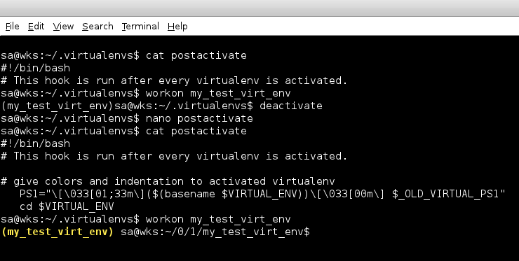
The currently active virtual environment is now yellow plus we got a
blank in between the yellow colored virtual environment and our
default prompt.
Another very handy thing I would recommend putting into postdeactivate
is cd $VIRTUAL_ENV (line 208) — it automatically beams us into the
virtual environment's root when we activate it i.e. no more need for
using cdvirtualenv right after workon <foo>.
Since PIP is used by pretty much anybody these days, here is how we
make virtualenv/virtualenvwrapper and PIP complement each other
nicely, thus providing for enhanced user experience:
sa@wks:~$ grep -A8 '\. pip' .bashrc
###_ . pip
export PIP_DOWNLOAD_CACHE=$HOME/.pip/cache
export PIP_SOURCE_DIR=$HOME/.pip/source
export PIP_BUILD_DIR=$HOME/.pip/build
export PIP_VIRTUALENV_BASE=$WORKON_HOME
export PIP_REQUIRE_VIRTUALENV=true
sa@wks:~$
This makes PIP use a local cache directory, thus save us time and
bandwidth and also allows us to work offline to some degree e.g. while
on a plane without Internet connectivity. We also have a directory to
store source code downloaded with PIP (which is what we use when we
decide to use so-called editable packages e.g. those are taken
directly from some GIT repository which updates we want to follow). Of
course, in some cases we need to compile/build source code so we also
have a build directory.
Next it detects an active virtual environment and install to it,
without having to pass it the -E switch plus it tells PIP to bail out
if we currently do not have a virtual environment activated — the
last one (PIP_REQUIRE_VIRTUALENV) is some sort of precaution in order
to avoid doing something silly to our global Python context/space.
Django Environment
This one I love! So far we have seen how to create virtual
environments. We even use virtualenvwrapper to make it a joy to work
with those virtual environments.
We create all kinds of Python projects atop/inside those virtual
environments e.g. we can test our code with different Python versions
like for example 2.7 and 3.2 by simply switching back and forth with
workon 2.7 and workon 3.2 respectively. We can test our Django
application with different third party applications... the things we
can do are literally endless...
However, while creating virtual environments is now easy and fast
(mkvirtualenv), creating a Django project still is quite a bit work —
all the pip install django, django-admin startproject, pip install
django-extensions, pip install fabric, etc. stuff... more so even the
creation of things like aliases and its dynamic enabling/disabling of
scoping based on what the current virtual environment is, symmetrical
links and all other custom things we might have in place. Gosh, we do
not want that tedious repetitive work no more... the solution to this
problem is with django-environment!
Virtualenv-Commands
So far I am not using it but from what I have seen it is pretty cool
too. Please go here and here for more information.
Detect a Virtualenv
Even though the idea behind a virtual environment is to be
transparent, there might be cases when we want to detect a virtual
environment i.e. whether or not we run inside one or not. Here is how
if sys.real_prefix:
print("We are inside a virtualenv.")
This checks for the existence of sys.real_prefix from a virtualenv's
modified site.py —
sys.real_prefix only exists with a virtual
environment but not with a normal/standard Python installation.
Virtualenv + GIT + Bash Prompt
We already know how to display information related to the current
virtual environment inside our Bash prompt. If, in addition, we want
to have GIT related information as well, we can do so easily. Here is
what it looks like:
 |
| blue is GIT related information, yellow is virtual environment related information |
PIP
... the Python installation tool PIP is an acronym for pip installs
packages, while technically the tool installs distributions, the name
package is used as its meaning is more widely understood. Even the
site where distributions are distributed at is called the
Python Package Index rather than Python Distribution Index.
WRITEME
Bash Completion
In order to have Bash completion with PIP, here is what we do:
- issue
pip completion --bash and
- put its output into
~/.bashrc which then looks like this
sa@wks:~$ grep -A7 "^_pip_completion()" .bashrc
_pip_completion()
{
COMPREPLY=( $( COMP_WORDS="${COMP_WORDS[*]}" \
COMP_CWORD=$COMP_CWORD \
PIP_AUTO_COMPLETE=1 $1 ) )
}
complete -o default -F _pip_completion pip
sa@wks:~$
A quick source ~/.bashrc picks up the changes/additions to
all the stuff in my ~/.bashrc and we are good to go... TAB TAB ;-]
Editable Packages
Those are packages/applications we install using pip install -e e.g.
pip install -e git+git://github.com/pinax/pinax.git#egg=pinax
Distutils, Setuptools, Distribute
One should have read about the history of packaging before continuing
here.
python setup.py develop installs a package without moving it into
../site-packages/
Distribute
This is the one we recommend to use. It is the successor to
Setuptools, which itself has always been considered the better
Distutils.
GNU Emacs
Since GNU Emacs is my weapon of choice for pretty much any battle
these days, I would like to honor my good fellow by explicitly telling
a bit how I made the out of the box setup which Emacs provides for
Python programming even more cosy ;-]
Theory
Because sometimes knowing how to fly a plane is not enough but rather,
we need to know the physics involved and maybe even how to design the
engine.
Call by...
value? reference? Neither one is what Python does! Let us first have a
look at what those two evaluation schemes are and then how Python
differs.
Call-by-Value
Call-by-value evaluation (also known as pass-by-value) is the most
common evaluation strategy, used in languages as different as C/C++
and Scheme. C++ defaults to call-by-value evaluation but offers to use
call-by-reference where/when needed/desired.
In call-by-value, the argument expression is evaluated, and the
resulting value is bound to the corresponding variable in the function
(frequently by copying the value into a new memory region) — a
pictures example of this can be seen here.
If the function or method is able to assign values to its parameters,
only its local copy is assigned i.e. everything passed into a function
call is unchanged in the caller's scope when the function returns.
Call-by-Reference
In call-by-reference evaluation (also known as pass-by-reference), a
function receives an implicit reference to the argument, rather than a
copy of its value.
This means that a function or method can modify the argument and thus
the value in the caller's scope. Call-by-reference therefore has the
advantage of greater time- and space-efficiency (values do not need to
be copied in memory), as well as the potential for greater
communication between a function/method and its caller (the
function/method can return information using its reference arguments),
but the disadvantage that a function must often take special steps to
protect values it wishes to pass to other functions.
Perl for example defaults to call-by-reference whereas others such as
C++ default to call-by-value but offer means to use call-by-reference.
Call-by-Sharing
What Python does is called call-by-sharing also known as
call-by-object-reference. So how is this different from call-by-value
and call-by-reference? Well, it is both, somewhat...
- assignments are call-by-value
-
The semantics of call-by-sharing differ from call-by-reference in that
assignments to function/method arguments within the function/method
are not visible in the caller's scope — same thing as with
call-by-value but unlike call-by-reference semantics.
- mutations are call-by-reference
-
However, since the function/method has access to the same object as
the caller (no copy is made), mutations to those objects within the
function/method become visible in the caller's scope — same thing as
call-by-reference but unlike call-by-value semantics. This behavior is
the reason why we should
never use mutable values as default parameter values.
The reason why people often confuse what Python does (call-by-sharing)
with call-by-value and/or call-by-reference may be due to the fact
that, in Python, the value of a name is a reference to an object i.e.
we always pass the value (no implicit copying), and that value is
always a reference — call-by-object-reference...
Since Python is a dynamically typed language, Python values (actually
objects — in Python everything is an object, remember?), not
variables, carry type. This has implications for many aspects of the
way the language behaves e.g. the way default parameter values behave.
All variables in Python hold references to objects, and these
references are passed to functions/methods. A function/method cannot
change the value a variable references in its calling function.
Type System
Before we start, there are some terms we need to know:
- The process of verifying and enforcing the constraints of types is
called type checking.
- A programming language is said to be dynamically typed (has a
dynamic type system) when type checking is performed at run time
as opposed to compile time.
- A type system is said to be strongly typed when it has
restrictions on operations involving values of different data
types e.g. Python does not allow to add a string to a number (e.g.
an integer).
- Dynamic binding also known as late binding means determining the
exact implementation of a request based on both the request
(operation) name and the receiving object at run time.
Python has a dynamic type system. However, despite having a dynamic
type system, Python is strongly typed, forbidding operations that are
not well-defined like, for example, adding a number to a string.
Being a dynamically typed language means name resolution is made
through dynamic binding also known as late binding i.e. name
resolution happens during run time. In other words, Python binds
method and variable names during program execution rather than at
compile time.
Functional Programming
WRITEME
Functions in Python are so-called First-Class objects.
Inversion of Control
- http://en.wikipedia.org/wiki/Inversion_of_control
- In traditional programming the flow of the business logic is
controlled by a central piece of code, which calls reusable
subroutines that perform specific functions. Using Inversion of
Control this central control design principle is abandoned. The
caller's code deals with the program's execution order, but the
business knowledge is encapsulated by the called subroutines.
- It is still undecided if Inversion of Control is a design pattern,
an architectural principle, or both.
- The need for reducing the number of configuration steps for
assembling a computing grid, as well as supporting adding nodes and
distributing computation to them as quickly as possible, also
drives the Colony Distributed initiative.
- distributing computation via virtual distribution: Viral
distribution, as per the Colony interpretation, would mean that a
configured Colony instance could make its computing power
available to a Colony managed computing grid, by announcing its
specifications, after which it would receive work units in the
form of plugins, i.e., mobile code for execution on the instance.
Introspection
Introspection is source code looking at source code e.g. other modules
and functions in memory as objects, getting information about them,
and manipulating them. In general, in computing, type introspection is
a capability of some object-oriented programming languages to
determine the type of an object at run time.
WRITEME
Aspect Oriented Programming
WRITEME
Metaprogramming
Metaclass
Please go here.
Abstract Class, Abstract Superclass
Please go here for more information.
Reflection
Lazy vs Greedy Evaluation
WRITEME
Protocol
Parallelism
WRITEME
Global Interpreter Lock
A GIL (Global Interpreter Lock) is a mutual exclusion lock held by an
interpreter thread. Its use is to avoid sharing code that is not
thread-safe with other threads.
There is always one GIL for one interpreter process. Problem is, while
this gives better performance on single-core machines, it fails to
scale for multiprocessor machines.
Even though that with CPython we are stuck with the GIL, there are
projects trying to get rid of the GIL — examples are Unladen Swallow
and Stackless Python.
Last but not least, even with CPython, the GIL might not be as much of
a problem as many think as we can have several ways for parallelism
even with CPython.
Design Patterns
A design pattern is a general reusable solution to a commonly
occurring problem in software design.
— Wikipedia
This is a huge subject, ready to fill bookshelves on its own. This
subsection will look at design patterns at code-level with regards to
Python i.e. not all known design patterns exist in Python respectively
make sense using them when programming in Python (this is true for any
other language as well).
Design patterns can be divided into several categories: Creational
Patterns, Structural Patterns, Behavioral Patterns and Concurrency
Patterns. They are described using the concepts of delegation,
aggregation, and consultation.
There also exists another classification that has the notion of
architectural design patterns which may be applied at the architecture
level of the software such as the MVC (Model-View-Controller) pattern.
This high-level view on design patterns is not covered here.
WRITEME
Creational Pattern
Creational design patterns are design patterns that deal with object
creation mechanisms, trying to create objects in a manner suitable to
the situation. The basic form of object creation could result in
design problems or added complexity to the design. Creational design
patterns solve this problem by somehow controlling this object
creation.
Singleton / Borg
Any type of which only one instance exists at all times is called a
singleton. One example of a singleton is None.
- Example
-
Say we had a class called
Sheep and use it to only instantiate one
sheep from it. We call this sheep ladygaga. ladygaga is our only
sheep. ladygaga is a singleton. ladygaga is alone in this world and
will be so forever. When ladygaga dies we might instantiate another
sheep, she really needs to be dead though... there can only be one
... sheep... at all times.
Factory
Mixin
Generally, in OOP (Object-Oriented Programming) languages, a mixin is
a class/type that provides a certain functionality to be inherited or
just reused by a subclass/subtype, while not meant for instantiation.
Inheriting from a mixin is not a form of specialization but is rather
a means of assembling features/functionality, something that can also
be achieved through composition (which in fact is mostly the better
way to assemble features/functionality).
A class/type may inherit most or all of its features/functionality
from one or more mixins through multiple inheritance. Of course, only
programming languages that support multiple inheritance allow us to do
mixins but that is implicit to the cause. Let me just make a short
note on mixins in Ruby:
-
Ruby is a single inheritance language, still Ruby has mixins. So, was
all I just said a lie? Nope... Mixins in Ruby are monkeypatches but
no proper mixins. The Ruby folks may call it a mixin, but it is a
different kind of thing.
So what is the difference between a mixin and multiple inheritance? Is
it just a matter of semantics and use? Yes, the difference between a
mixin and multiple inheritance is in fact just a matter of semantics
i.e. if we create a class/type using multiple inheritance then we
might as well utilize mixins by subclassing from them, thus assembling
features/functionality in our class/type. We ultimately end up with
the assembly of features/functionality contained in all mixins and
everything we put into this particular class/type itself.
Mixins encourage the DRY (Don't repeat yourself) principle (code
reuse) because they can be used in two ways:
- We want to have optional features/functionality, which may or may
not be added to a particular class/type (example of
Foo and Bar
below).
- We want to have particular features/functionality in more than one
class/type.
We are now going to use the socketserver module, which has both, a
UDPServer as well as a TCPServer class/type which act as a server for
UDP (User Datagram Protocol) and TCP (Transmission Control Protocol)
socket servers respectively — by default all new connections are
handled within the same process.
However, additionally, there are two mixin classes/types: ForkingMixIn
and ThreadingMixIn. By extending TCPServer with the ThreadingMixIn
like shown below, the ThreadingMixIn class/type adds optional
features/functionality to the TCPserver class/type such that each new
connection creates a new thread. Alternatively, using the ForkingMixIn
would cause the process to be forked for each new connection.
Clearly, the functionality to create a new thread or fork a process is
not terribly useful as a stand-alone class/type but very much so when
used as a mixin. Also, just to mention/demonstrate it, there is
ThreadingTCPServer, a ready-made class/type that can be used by us
straight away when in fact it is the same as our Foo class/type where
we did the extra step manually:
>>> import socketserver
>>> socketserver.__all__
['TCPServer', # the base class/type we are going to use
'UDPServer',
'ForkingUDPServer',
'ForkingTCPServer',
'ThreadingUDPServer',
'ThreadingTCPServer', # ready-made class/type
'BaseRequestHandler',
'StreamRequestHandler',
'DatagramRequestHandler',
'ThreadingMixIn', # the threading mixin, the mixin we chose
'ForkingMixIn',
'UnixStreamServer',
'UnixDatagramServer',
'ThreadingUnixStreamServer',
'ThreadingUnixDatagramServer']
Let us have a look at the ready-made class/type first — its
superclass/supertype as well as its MRO (Method Resolution Order):
>>> socketserver.ThreadingTCPServer.__bases__
(<class 'socketserver.ThreadingMixIn'>, <class 'socketserver.TCPServer'>)
>>> socketserver.ThreadingTCPServer.mro()
[<class 'socketserver.ThreadingTCPServer'>,
<class 'socketserver.ThreadingMixIn'>,
<class 'socketserver.TCPServer'>,
<class 'socketserver.BaseServer'>,
<class 'object'>]
>>> class Bar(socketserver.ThreadingTCPServer):
... pass
...
...
>>> Bar.__bases__
(<class 'socketserver.ThreadingTCPServer'>,)
>>> Bar.mro()
[<class '__main__.Bar'>,
<class 'socketserver.ThreadingTCPServer'>,
<class 'socketserver.ThreadingMixIn'>,
<class 'socketserver.TCPServer'>,
<class 'socketserver.BaseServer'>,
<class 'object'>]
Now with the extra manual step of building a class/type that is
semantically the same as Bar:
>>> class Foo(socketserver.ThreadingMixIn, socketserver.TCPServer):
... pass
...
...
>>> Foo.__bases__
(<class 'socketserver.ThreadingMixIn'>, <class 'socketserver.TCPServer'>)
>>> Foo.mro()
[<class '__main__.Foo'>,
<class 'socketserver.ThreadingMixIn'>,
<class 'socketserver.TCPServer'>,
<class 'socketserver.BaseServer'>,
<class 'object'>]
>>>
Marvelous! Foo and Bar are the same (except for the difference in the
first class/type with the MRO but that is to be expected of course).
What we have done is use the ThreadingMixIn mixin to provide optional
underlying features/functionality without affecting the main
features/functionality as a socket server.
Trait
Traits are a simple composition mechanism for structuring
object-oriented programs. A trait is essentially a parameterized set
of methods which serves as a behavioral building block for
classes/types and is the most basic unit of code reuse.
With traits, classes/types are still organized in a single inheritance
hierarchy, but they can make use of traits to specify the incremental
difference in behavior with respect to their superclasses/supertypes.
Unlike mixins and multiple inheritance, traits do not employ
inheritance as the composition operator. Instead, trait composition is
based on a set of composition operators that are complementary to
single inheritance and result in better composition properties.
In short: A trait is a bunch of methods and attributes with the
following characteristics:
- the methods/attributes in a trait belong logically together.
- if a trait enhances a class/type, then all subclasses/subtypes are
enhanced too.
- if a trait has methods in common with the class/type, then the
methods defined in the class/type have precedence.
- the trait order is not important i.e. enhancing a class/type first
with trait T1 and then with trait T2 or vice versa is the same.
- if traits T1 and T2 have names in common, enhancing a class both
with T1 and T2 raises an error.
- if a trait has methods in common with the superclass/supertype,
the trait methods have precedence.
- a class/type can be seen both as a composition of traits and as an
homogeneous entity.
Characteristics from 4 to 7 are the distinguishing characteristics of
traits with respect to multiple inheritance and mixins. In particular,
because of 4 and 5, all the complications with the MRO (Method
Resolution Order) disappear and the overriding is never implicit.
Property 6 is mostly unusual — typically in Python the
superclass/supertype has the precedence over mixin classes. Property 7
should be intended in the sense that a trait implementation must
provide introspection facilities to make seemless the transition
between classes viewed as atomic entities and as composed entities.
Resource Acquisition Is Initialization
Structural Pattern
Structural design patterns are design patterns that ease the design by
identifying a simple way to realize relationships between entities.
Facade
Proxy
Adapter
What an adapter does is wrap a class/type foo or an instance thereof
so that it works/behaves in a context intended for class/type bar or
an instance thereof. See decorator vs adapter for more information.
Decorator
See decorator and decorator vs adapter.
Behavioral Pattern
Behavioral design patterns are design patterns that identify common
communication patterns between objects and realize these patterns. By
doing so, these patterns increase flexibility in carrying out this
communication.
State Pattern
Delegation
Strategy
Chain of Responsibility
Observer
Visitor
Template
Concurrency Pattern
Concurrency patterns are those types of design patterns that deal with
multi-threaded programming paradigm.
Actor Model
Miscellaneous
This section provides miscellaneous information within regards to
Python.
Manual Install
Here is how we manually install Python from trunk/HEAD/tip (or
whatever one may call it; read most-current or up-to-date) on Debian
at a filesystem location of our choosing (it usually installs to
/usr/local/* but we will choose /tmp for this example). We start by
installing a bunch of necessary packages for the build process.
Another maybe simpler way would be to issue aptitude build-dep python
and let APT figure out and install all the packages needed:
sa@wks:~$ su
Password:
wks:/home/sa# lsb_release -a
No LSB modules are available.
Distributor ID: Debian
Description: Debian GNU/Linux unstable (sid)
Release: unstable
Codename: sid
wks:/home/sa# cd /tmp; aptitude install git mercurial build-essential zlib1g-dev libreadline-dev libncursesw5-dev libncurses5-dev libsqlite3-dev mime-support libbz2-dev
[skipping a lot of lines...]
wks:/tmp# hg clone http://hg.python.org/cpython # here we clone the Python Mercurial repository
destination directory: cpython # once cloned "hg pull -u" would pull in new changes
requesting all changes
adding changesets
adding manifests
adding file changes
added 73394 changesets with 164534 changes to 9371 files (+1 heads)
updating to branch default
3716 files updated, 0 files merged, 0 files removed, 0 files unresolved
wks:/tmp# date -u; cd cpython
Sun Nov 6 01:33:06 UTC 2011
wks:/tmp/cpython# ./configure --prefix=/tmp/python-$(date +%s) # let us put a timestamp here
checking for hg... found
checking for --enable-universalsdk... no
checking for --with-universal-archs... 32-bit
[skipping a lot of lines...]
creating Modules/Setup.local
creating Makefile
wks:/tmp/cpython# make && make install
gcc -pthread -c -Wno-unused-result -DNDEBUG -g -fwrapv -O3 -Wall -Wstrict-prototypes -I. -I./Include -DPy_BUILD_CORE -o Modules/python.o ./Modules/python.c
gcc -pthread -c -Wno-unused-result -DNDEBUG -g -fwrapv -O3 -Wall -Wstrict-prototypes -I. -I./Include -DPy_BUILD_CORE -o Parser/acceler.o Parser/acceler.c
[skipping a lot of lines...]
(cd /tmp/python-1320543270/bin; ln -s 2to3-3.3 2to3)
rm -f /tmp/python-1320543270/bin/pysetup3
(cd /tmp/python-1320543270/bin; ln -s pysetup3.3 pysetup3)
wks:/tmp/cpython# cd ..
wks:/tmp# cd python-1320543270/
wks:/tmp/python-1320543270# date -d @1320543270
Sun Nov 6 01:34:30 GMT 2011
wks:/tmp/python-1320543270# date -d @$(date +%s)
Sun Nov 6 01:40:02 GMT 2011 # compiling took roughly six minutes
wks:/tmp/python-1320543270# ./bin/python3 -c 'import sys; print(sys.version)'
3.3.0a0 (default:992ba03d60a8, Nov 6 2011, 01:37:15)
[GCC 4.6.2]
wks:/tmp/python-1320543270# type la; la
la is aliased to `ls -la'
total 24
drwxr-xr-x 6 root root 4096 Nov 6 01:38 .
drwxrwxrwt 41 root root 4096 Nov 6 01:45 ..
drwxr-xr-x 2 root root 4096 Nov 6 01:38 bin
drwxr-xr-x 3 root root 4096 Nov 6 01:38 include
drwxr-xr-x 4 root root 4096 Nov 6 01:38 lib
drwxr-xr-x 3 root root 4096 Nov 6 01:38 share
wks:/tmp/python-1320543270# echo 'that is it... we just build ourselves a bleeding-edge up-to-date Python :)'
that is it... we just build ourselves a bleeding-edge up-to-date Python :)
wks:/tmp/python-1320543270#
Debian
This subsection is intended to cover Debian specifics with regards to
Python.
../dist-packages
Before we actually answer that, let us have a look at the big picture
of having public and private installations of Python modules and
packages. Let us also have a glance at the difference about the main
Python installations (also known as global Python context/space) and
virtual environments:
By default Python modules/packages are searched in the current working
directory first, next in the directories listed in the PYTHONPATH
environment variable and finally all directories listed in the
sys.path Python variable are searched. That is just half the truth
actually...
The full truth is that Python initializes sys.path from PYTHONPATH and
that it includes the current working directory — however, once
Python's machinery gets going, PYTHONPATH and the current working
directory are ignored.
That said, there are generally three ways to install Python
modules/packages — there are public ones and private ones with
regards to the systems main Python installation (also known as global
Python context/space) and then there are virtual environments which
are either clones of the global Python context/space or which are
entirely separated Python contexts/spaces on their own:
- Public modules/packages are installed in a public directory as
listed in the afore mentioned
PYTHONPATH environment variable or
in directories found in sys.path.
- Directories with private Python modules/packages must be absent
from both,
PYTHONPATH and sys.path, so to not being picked up. In
case we want/need paths providing private Python modules/packages
which cannot be seen from the global Python context/space, they
should be installed in a private directory such as
/usr/share/<package-name> or /usr/lib/<package-name> for example
(paths not listed in sys.path and/or PYTHONPATH) where they are
generally only accessible to a specific program or suite of
programs included in the same package.
- Another way to have modules/packages installed would be to use a
virtual environment.
Right now we are only looking at the global Python context/space and
leave aside virtual environments. We are also just looking at the
public modules/packages subset and not how to handle private
modules/packages within the global Python context/space.
Finally, why Debian has ../dist-packages directories:
The installation location for Python code packaged by Debian is the
system Python modules directory, /usr/lib/pythonX.Y/dist-packages for
Python 2.6 and later, and /usr/lib/pythonX.Y/site-packages for Python
2.5 and earlier. In other words, whenever we use APT (Advanced
Packaging Tool) to install Python software, things land in
/usr/lib/pythonX.Y/dist-packages.
Tools used for packaging Python source code for Debian like
python-central and python-support take care of using the correct path
automatically. As an exception, modules managed by python-support are
installed in another directory which is added to sys.path using the
.pth files mechanism.
In case we are on Python 2.6 or later and do not use APT but some
other means (e.g. EasyInstall, PIP, etc.) to install public Python
code, /usr/local/lib/pythonX.Y/dist-packages is used. In case of
Python 2.5 or earlier the path would change to
/usr/local/lib/pythonX.Y/site-packages. This however is problematic
since, for Python 2.5 and earlier, this directory is also visible to
the default installation of Python and could thus lead to clashes if
the same Python module/package was installed via APT as well as
manually using PIP, EasyInstall etc. In order to avoid those clashes
Debian has introduced its ../dist-packages directories which helps
avoid those clashes.
When binary packages ship identical source code for multiple Python
versions, for instance /usr/lib/python3.1/dist-packages/foo.py,
/usr/lib/python2.6/dist-packages/foo.py and
/usr/lib/python2.5/site-packages/foo.py, these should point to a
common file. A common location to share, across Python versions,
arch-independent files which would otherwise go to the directory of
system public modules is /usr/share/pyshared.
Summary
The below is true for Python 2.6 and bigger
- If we install some Python software which is packaged by Debian,
/usr/lib/pythonX.Y/dist-packages is where stuff goes. This
directory may also contain some .pth files which contain additional
paths which will be appended to sys.path.
- In case we install Python software manually (using EasyInstall,
PIP, etc.) things go to
/usr/local/lib/pythonX.Y/dist-packages.
- Identical Python binaries for two or more versions of Python go to
/usr/share/pyshared.
Note the difference between /usr/lib/.. and /usr/local/lib/... More
information can be found in /usr/lib/pythonX.Y/site.py —
read the
code.
Monkey Patching
A monkey patch is a way to extend and/or modify the run-time code of
dynamic languages such as Smalltalk, JavaScript, Objective-C, Ruby,
Perl, Python, Groovy, etc. without altering its on-disk source code.
In Python, the term monkey patch only refers to dynamic modifications
of a class/type at run time based on the intent to patch existing
methods in an external class as a workaround to a bug and/or feature
which does not act as we desire. Examples of using monkey patching are
- Replace methods/attributes/functions at run time e.g. to stub out a
function during testing.
- Modify/extend behavior of a third-party product without
maintaining a private copy of the source code.
- Apply a patch at run time to the objects in memory, instead of the
on-disk source code.
- Distribute security and/or behavioral fixes that live alongside
the original on-disk source code (an example of this would be
distributing the fix as a plugin for the Ruby on Rails platform).
In general however it is fair to say that one should refrain from
monkey patching since it mostly introduces more problems than it
solves.
- Features/fixes made through monkey patching almost never get
documented, it is the oh-so-well-known quick hack/fix...
- They can lead to upgrade problems when the patch makes assumptions
about the patched object that are no longer true e.g. if the
product we have changes with a new release it may very well break
our patch. For this reason monkey patches are often made
conditional, and only applied if appropriate.
- If two modules attempt to monkey-patch the same method, one of them
(whichever one runs last) wins and the other patch has no effect,
unless monkeypatches are written with pattern like
alias_method_chain.
- They create a discrepancy between the original on-disk source code
and the observed behavior that can be very confusing to anyone
unaware of the patche's existence.
Even if monkey patching is not used, many people see a problem with
the availability of the feature, since the ability to use monkey
patching in a programming language is incompatible with enforcing
strong encapsulation, as required by the object-capability model,
between objects. Bottom line is, one should not use monkey patching
for the afore mentioned reasons and many more...
Magic Number
The magic number from Unix-like operating systems where the first few
bytes of a file hold a marker indicating the file type. It tells the
operating system whether or not the file is a binary executable, and
if so, which of several types thereof. The file command can be used to
read that information
1 sa@wks:/tmp$ echo "some text" > mytextfile
2 sa@wks:/tmp$ file my*
3 myimage.png: PNG image data, 2560 x 1600, 8-bit/color RGB, non-interlaced
4 mytextfile: ASCII text
5 sa@wks:/tmp$ mv myimage.png myblabla.txt
6 sa@wks:/tmp$ file myblabla.txt
7 myblabla.txt: PNG image data, 2560 x 1600, 8-bit/color RGB, non-interlaced
8 sa@wks:/tmp$
File extensions and name do not matter, only the magic number matters
as can be seen from lines 3 and 7, where we are actually looking at
the same file which only happens to have different names and file
extensions.
So, what does all this have to do with Python one might ask? Well,
Python puts a similar marker into its bytecode (.pyc) files when it
creates them.
The Python interpreter then makes sure this number is correct when
loading it. Anything that damages this magic number will cause a
problem like for example
Traceback (most recent call last):
File "amman.001", line 3, in <module>
ImportError: Bad magic number in..........amman.pyc
Things that could cause such damage include things like editing the
.pyc file or trying to run a .pyc from a different version of Python
(usually later) than our current interpreter version. There are things
we can do to avoid such errors/problems.
If they are our own .pyc files then the task becomes easy as all we
have to do is to delete them and let the interpreter re-compile the
.py files into new .pyc files. A command to get rid of all .pyc files
in the current directory and all of its children (read recursively) is
find </path/to/root/of/.pyc_files> -type f -name "*.pyc" -exec rm {}
\;.
However, if they are not ours, we will have to either get the .py
files or an interpreter that can run the .pyc files with that
particular magic number (see below).
One thing worth noting here is that, as it often happens, we might see
such problem only occur under certain circumstances e.g. with lazy
imports .pyc files may only be imported under certain conditions based
only on the fact on whether or not their functionality is needed by
the current run-time environment.
Magic Numbers in Python
As mentioned, different versions of the Python interpreter have
different magic numbers. The list of all magic numbers can be found in
../Python/import.c:
sa@wks:~/0/python/py3/Python$ grep -A51 "Known values" import.c
Known values:
Python 1.5: 20121
Python 1.5.1: 20121
Python 1.5.2: 20121
[skipping a lot of lines...]
Python 3.2a0: 3160 (add SETUP_WITH)
tag: cpython-32
Python 3.2a1: 3170 (add DUP_TOP_TWO, remove DUP_TOPX and ROT_FOUR)
tag: cpython-32
Python 3.2a2 3180 (add DELETE_DEREF)
sa@wks:~/0/python/py3/Python$ date -u
Wed Feb 2 10:44:13 UTC 2011
sa@wks:~/0/python/py3/Python$
Sorting and Searching
Time
Time is an important subject, in general, and of course also for
programmers and technicians like us. Python's standard library ships a
few modules (time, datetime and calendar) that help us with all kinds
of time-related tasks in Python... set it, read it, store it,
manipulate it... People have also written many third-party modules
such as python-dateutil which provide us with additional features such
as enhanced mathematical operations on datetime objects.
naive, aware
There are two kinds of date and time objects in Python: naive and
aware. This distinction refers to whether the object has any notion of
timezone, DST (Daylight Saving Time), or other kind of algorithmic or
political time adjustment.
Whether a naive date/time object represents UTC (Universal Time
Coordinated), local time, or time in some other timezone is purely up
to the program, just like it is up to the program whether a particular
number represents metres, miles, or mass. Naive date/time objects are
easy to understand and to work with, at the cost of ignoring some
aspects of reality.
Daylight Saving Time, UTC, GMT
DST is this bizarre thing of moving clocks back and forth twice a
year. This happens roughly at the same time in most countries but
there are of course many exceptions which makes the whole notion of
DST even more silly. Python's datetime module allows us to deal with
this and keep our sanity whenever we need to expose date/time
information externally.
Roughly speaking, UTC is the better/newer GMT (Greenwich Mean Time),
that is all we need to know when it comes to coding really. Quite
often however the terms are used interchangeably e.g. the gmtime()
function from the time module carries the name gm when really it
should be named utctime() in my opinion.
We should always determine and store time in UTC —
storing time as
local time, its offset to UTC and whether or not DST is in effect
should be avoided as it is a recipe for confusion and errors. If we
need to record where time was taken then we store the offset to UTC,
the timezone name, and whether or not DST is in effect separately and
apply this information whenever date/time is exposed externally e.g.
to a user.
In other words: we always deal with UTC-based date/time values/objects
internally and only map to local representation and/or DST when date
and/or time exposed externally e.g. shown to a user.
Do:
- Always store time according to a unified standard that is not
affected by DST (e.g. UTC).
- Include the local time offset to UTC as is (including DST offset)
when storing timestamps. The
timezone class/type from the datetime
module is well-suited for this job.
- Include the original timezone name, so you can reconstruct the
original time at a later point and display correct offsets if
needed. Again, the
timezone class/type is perfect here.
- Remember that DST offsets are not always an integer number of hours
e.g. Indian Standard Time is UTC+05:30.
- Internal logic should always work on UTC-based dates/times.
- Keep timestamps in seconds since epoch e.g. as returned by the
time() function from the time module.
- Only convert to local times and/or DST at the last possible moment
before exposing it externally.
- Remember that timezones and offsets are not fixed and may change.
For instance, historically US and UK used the same dates to spring
forward and fall back. However in the mid 2000's the US changed the
dates that the clocks get changed on. This now means that for 50
weeks of the year the difference is 5 hours and for 2 weeks it is 4
hours. Be aware of items like this in any calculations that involve
multiple zones.
- Keep OS, database and application tzdata files in sync, between
themselves and the rest of the world.
- Set hardware clocks and OS clocks to UTC using NTP (Network Time
Protocol) services such as
chrony on Debian.
- Store server time, not client time.
- When dealing with recurring events (weekly TV show, for example),
remember that the time changes with DST and will be different
across time zones.
- Lobby to end the abomination that is DST. We can always hope...
Do Not:
- Do not use JavaScript date and time calculations in web
applications unless you absolutely have to.
- Never trust dates/times coming from non-server sources e.g. a
user's web browser.
- For the same reasons, do not compare client dates/times with server
dates/times.
ISO 8601
2012-11-22 14:46:27 is how we should represent date and time these
days no matter where we are on this planet and which
cultural/political audience we expect. ISO 8601 is the new
international standard which is recommended over older national
standards such the American way of writing 11/22/12 for November 22nd
2012 for example. Here is how we get an ISO 8601 date/time
representation in Python:
>>> from time import strftime
>>> strftime("%Y-%m-%d %H:%M:%S") # time module
'2011-10-29 21:06:40'
>>> from datetime import datetime
>>> str(datetime.now()).split('.')[0] # datetime module
'2011-10-29 21:06:46'
>>> "{:%Y-%m-%d %H:%M:%S}".format(datetime.now()) # using .format() string method
'2011-10-29 21:06:51'
>>>
time vs datetime
The datetime module provides a number of classes/types to deal with
dates, times, and time intervals and can be thought of as successor to
the integer/tuple-based time module as it provides a more
object-oriented interface.
That being said, time is useful for non-complex time-based operations,
especially when doing system administration and automation tasks such
as encoding directory creating time in the directory name, putting
timestamps in log files...
time
The time module uses two different representations for a point in time
and provides numerous functions to help us convert back and forth
between the two:
- a float number: This is the UNIX internal representation for time
also known as the Unix epoch (seconds elapsed since 1970-01-01
00:00:00). In this representation, a duration between points in
time is also a float number.
- a
struct_time object: This object has nine attributes for
representing a point in time as a Gregorian calendar date/time. In
this representation, there is no representation for the duration
between points in time, we need to convert back and forth between
struct_time and seconds/float representations.
One of the core functions of the time module is time(), which returns
the number of seconds since the Unix epoch as a floating point value:
Wall Clock Time vs Processor Time
>>> import time
>>> time.time()
1320009370.628919 # seconds since Unix epoch (1970-01-01 00:00:00)
>>> type(time.time())
<class 'float'> # type float
>>> int(time.time()) # seconds resolution as integer is easier to work with
>>> 1320009378
>>> time.ctime()
'Sun Oct 30 21:22:43 2011' # non-ISO 8601 string representation
Although the value is always a float, actual precision is
platform-dependent. The float representation is useful when storing or
comparing times internally, but not as useful for showing it
externally e.g. to a user. In that case it makes more sense to use
ctime() or strftime() in case we want to do the right thing and format
time in ISO 8601:
While time() and ctime() return a wall clock time, clock() returns
processor clock time. The values returned from clock() should be used
for performance testing, benchmarking, etc. since they reflect the
actual time used by the program, and can be more precise than the
values from time():
>>> import time
>>> def worker():
... for i in range(1000000):
... i += i/2
...
...
...
>>> def using_time():
... start = time.time()
... worker()
... print("elapsed time: {}".format(time.time() - start))
...
...
>>> def using_clock():
... start = time.clock()
... worker()
... print("elapsed time: {}".format(time.clock() - start))
...
...
>>> using_time()
elapsed time: 1.7183270454406738
>>> using_clock()
elapsed time: 1.6999999999999886
>>>
Although both, time() and clock() can be used for benchmarking, rule
of thumb is: clock() is better than time() but using the timeit module
is best because it has the best resolution and its results are the
least platform dependent.
Timezones
>>> time.tzname
('GMT', 'BST') # I am currently in London therefore
>>> time.timezone
0 # local time and UTC is the same in my case
>>> time.daylight
1 # this timezone uses DST
>>> time.altzone
-3600 # current DST offset in seconds
>>> time.strftime('%Y-%m-%d %H:%M:%S', time.gmtime())
'2011-10-31 22:11:17' # ISO 8601 string representation
>>> time.strftime('%Y-%m-%d %H:%M:%S')
'2011-10-31 22:11:21' # ISO 8601 string representation
>>> time.ctime()
'Mon Oct 31 11:16:10 2011' # non-ISO 8601 string representation
>>>
If we wanted to return UTC then we could use gmtime() and supply it to
strftime() as shown above (they are the same in my case because I am
currently in the UK).
struct_time
Storing times as elapsed seconds is useful in some situations, but
there are times when we need to have access to the individual fields
of a point in time (year, month, etc.).
As mentioned, the time module has two different representations for a
point in time, the floating point based one which we have just seen
using time(), and struct_time, a named tuple with components broken
out so they are easy to access.
- Rule of thumb is that when we need to compute time between two
points in time then using the floating point representation is the
way to go.
- If on the other hand, if we need more detailed
information/operations on a point in time, then
struct_time is the
way to go as it has nine attributes such as tm_year which describe
a point in time.
There are several functions that work with struct_time values instead
of floats: gmtime(), localtime() (and its inverse mktime()), and
strptime() for example:
>>> time.gmtime()
time.struct_time(tm_year=2011, tm_mon=10, tm_mday=31, tm_hour=9, tm_min=39, tm_sec=55, tm_wday=0, tm_yday=304, tm_isdst=0)
>>> time.localtime()
time.struct_time(tm_year=2011, tm_mon=10, tm_mday=31, tm_hour=9, tm_min=40, tm_sec=4, tm_wday=0, tm_yday=304, tm_isdst=0)
>>> time.mktime(time.gmtime())
1320054020.0
>>> time.time()
1320054024.777523
>>> time.mktime(time.localtime()) # convert a struct_time to float
1320054095.0
>>> time.time()
1320054096.891176
>>> now = time.gmtime()
>>> now.tm_yday
304
>>> now.tm_year
2011
gmtime() returns the current time in UTC. localtime() returns the
current time with the current time zone applied (might be the same as
UTC if you are in the UK). mktime() takes a struct_time and converts
it to the floating point representation and strptime() takes a string
and parses it and returns a struct_time.
Parsing and Formatting Times
The two functions strptime() and strftime() convert between
struct_time and string representations of points in time. Below we
have the current time as a string, a struct_time instance, and another
but this time ISO 8601 string:
>>> now = time.ctime()
>>> now
'Mon Oct 31 10:49:41 2011' # non ISO 8601 string representation
>>> time.strptime(now)
time.struct_time(tm_year=2011, tm_mon=10, tm_mday=31, tm_hour=10, tm_min=49, tm_sec=41, tm_wday=0, tm_yday=304, tm_isdst=-1)
>>> time.strftime('%Y-%m-%d %H:%M:%S', time.strptime(now))
'2011-10-31 10:49:41' # ISO 8601 string representation
>>> time.strftime('%Y-%m-%d %H:%M:%S')
'2011-10-31 10:50:26' # ISO 8601 string representation
>>>
Those are just examples on how to use the time module and I always
prefer to use "{:%Y-%m-%d %H:%M:%S}".format(datetime.now()) whenever I
need ISO 8601 representation of date/time simply because it seems more
robust to use datetime in this case and also get the goodness of the
format() string method.
Miscellaneous
Last but not least, the time module has some more handy functions such
as sleep() up its sleeve:
>>> def sleep_example():
... print(time.time())
... time.sleep(2) # will delay processing for 2 seconds
... print(time.time())
...
...
>>> sleep_example()
1320055818.41326
1320055820.415575
>>>
datetime
The datetime module contains all of the objects and methods required
to correctly handle the sometimes obscure rules for the
Gregorian calendar. Additionally, it is possible to use date
information in the datetime object to convert among the world's
calendars.
- The
datetime module has just one representation for a point in
time as opposed to two as seen with the time module.
- It assigns an ordinal number to each day. The numbers are based on
an epochal date, and algorithms to derive the year, month and day
information for that ordinal day number.
- Similarly, this class/type provides algorithms to convert a
calendar date to an ordinal day number. Marginal note: the
Gregorian calendar was not defined until 1582, all dates before
the official adoption are termed proleptic. Further, the calendar
was adopted at different times in different countries.
As of now (November 2011) there are six classes/types in the datetime
module that help us handle dates and times in a uniform and correct
manner:
date: An idealized naive date, assuming the current Gregorian
calendar always was, and always will be, in effect.time: An idealized time, independent of any particular day,
assuming that every day has exactly 86400 seconds (there is no
notion of leap seconds here).datetime: A combination of a date and a time.timedelta A duration expressing the difference between two date,
time, or datetime instances to microsecond resolution.tzinfo: An abstract superclass for timezone information objects.
These are used by the datetime and time classes/types to provide a
customizable notion of time adjustment (for example, to account for
timezone and/or DST).timezone: A class/type that implements the tzinfo abstract super
class/type as a fixed offset to UTC.
Notes about those types:
- Objects of these types are immutable.
- Objects of the
date class/type are always naive.
- An object
foo of class/type time or datetime may be naive or aware.
foo is aware if foo.tzinfo is not None and
foo.tzinfo.utcoffset(foo) does not return None. If foo.tzinfo is
None, or if foo.tzinfo is not None but foo.tzinfo.utcoffset(foo)
returns None, foo is naive.
- The distinction between naive and aware does not apply to
timedelta
objects.
Class/Type relationships:
object
timedelta # no notion of naive/aware
tzinfo # an ABC; used by time and datetime objects
timezone # subclass/subtype of tzinfo
time # naive or aware
date # naive-only
datetime # naive or aware
We will now take a closer look at the datetime class/type of the
datetime module as it allows for combined time and date aware
operations:
>>> import datetime
>>> datetime.MINYEAR # constants exported by the datetime module
1
>>> datetime.MAXYEAR
9999
>>> now = datetime.datetime.now()
>>> now
datetime.datetime(2011, 10, 30, 1, 30, 51, 906080)
>>> repr(now)
'datetime.datetime(2011, 10, 30, 1, 30, 51, 906080)' # ISO 8601 representation
>>> print(now)
2011-10-30 01:30:51.906080 # print() returns __str__() if available, __repr__() otherwise
>>> str(now)
'2011-10-30 01:30:51.906080'
>>> str(now).split('.')[0]
'2011-10-30 01:30:51'
>>> now.second # instance attribute
51
>>> now.microsecond
906080
>>> now.year
2011
>>> now.year = 2021 # fails because instance attributes are read-only
Traceback (most recent call last):
File "<input>", line 1, in <module>
AttributeError: attribute 'year' of 'datetime.date' objects is not writable
>>> now.min # class attributes
datetime.datetime(1, 1, 1, 0, 0)
>>> now.max
datetime.datetime(9999, 12, 31, 23, 59, 59, 999999)
>>> now.resolution
datetime.timedelta(0, 0, 1)
Note that the default string representation of datetime instances is
an ISO 8601-style timestamp. time as well as datetime modules make use
of time.struct_time objects which we know provide named tuple
interfaces:
>>> datetime.datetime.timetuple(now)
time.struct_time(tm_year=2011, tm_mon=10, tm_mday=30, tm_hour=1, tm_min=30, tm_sec=51, tm_wday=6, tm_yday=303, tm_isdst=-1)
>>> type(datetime.datetime.timetuple(now))
<class 'time.struct_time'> # a named tuples give us
>> bar = datetime.datetime.timetuple(now)
>>> bar[0] # index-based as well as
2011
>>> bar.tm_year # name-based access
2011
>>> bar.tm_sec
51
>>> time.gmtime()
time.struct_time(tm_year=2011, tm_mon=10, tm_mday=30, tm_hour=19, tm_min=9, tm_sec=8, tm_wday=6, tm_yday=303, tm_isdst=0)
>>> type(time.gmtime())
<class 'time.struct_time'>
>>>
A time.struct_time object providing a named tuple interface is
returned by the gmtime(), localtime(), and strptime() functions from
the time module and the timetuple() and utctimetuple() methods on
instances of the datetime class/type from the datetime module.
There is much more to be found in the datetime module, especially with
regards to time/date arithmetic and timezone based tasks which makes a
closer look certainly worth the time! Also, as mentioned, the
third-party python-dateutil package is a good place to look for when
we need to do heavy time-based arithmetic which under normal
circumstances would get complex rather quickly.
Summary
- The
time module is basically for working with Unix timestamps
expressed as floating point numbers in seconds since the Unix epoch
(1970-01-01 00:00:00). Rather than being object oriented it works
of an integer/tuple-based time mechanism and as such only provides
a mere function-based API. The datetime module on the other hand
has an object oriented API and is more powerful and versatile and
most of the time easier to use because it only has one internal
representation for any point in time (as opposed to two with the
time module). datetime also provides support for timezones, DST and
many things the time module lacks. It is therefore recommended to
use the datetime module in most cases.
- Store time in UTC and always use UTC-based date/time values/objects
internally e.g. when doing date/time arithmetic — only map to its
local representation when it is exposed externally e.g. shown to a
user.
- It is recommended to use date/time aware objects (class/type
time
or datetime from the datetime module) to capture/represent
timezones, timezone names, and whether or not DST is in effect but
store this information in a way so that it becomes additional
information to actual UTC-based dates/times. This means we can use
UTC-based date/time internally and only have to map to timezone
and/or DST aware dates/times when we expose date/time information
externally.
- When exposing date/time externally, it is recommended to use modern
ISO 8601 representation.
Codecs
WRITEME
Tips and Tricks
This section is used to collect bits and pieces of mostly unrelated
bits and pieces. What they all have in common however is that they are
considered to be pythonic when it comes to pure coding and/or, they
all relate to Python in a certain way:
Find Code on the Filesystem
Using introspection we can use a module's __file__ attribute for that:
>>> import email
>>> email.__file__
'/home/sa/0/1/python3.3/lib/python3.3/email/__init__.py'
>>> import sys
>>> sys.__file__
Traceback (most recent call last):
File "<input>", line 1, in <module>
AttributeError: 'module' object has no attribute '__file__'
>>> sys.version
'3.3.0a0 (default:c33aa14f4edb, Nov 5 2011, 21:41:34) \n[GCC 4.6.2]'
>>>
The __file__ attribute contains the pathname of the file from which
the module was loaded, if it was loaded from a file. The attribute is
not present for C modules that are statically linked into the
interpreter (e.g. sys). For extension modules loaded dynamically from
a shared library, it is the pathname of the shared library file.
Python Version
Here is how we find out about which version of Python we are running:
sa@wks:~$ python
>>> import sys
>>> sys.version[:3]
'3.3'
>>> import platform
>>> platform.python_version()
'3.3.0a0'
>>> import sysconfig
>>> sysconfig.get_python_version() # available since Python 3.2
'3.3'
>>>
sa@wks:~$ python --version
Python 3.3.0a0
sa@wks:~$ python -c "import sys; print(sys.version)"
3.3.0a0 (default:c33aa14f4edb, Nov 5 2011, 21:41:34)
[GCC 4.6.2]
sa@wks:~$
Underscore / Interactive Interpreter
The name or identifier _ (a single underscore) is special in
interactive interpreter sessions as the interpreter binds _ to the
result of the last expression/statement it has evaluated, if any.
sa@wks:~$ python
>>> 2 + 2
4
>>> _
4
>>> _ + 2
6
>>> _ + 3
9
>>> print(_)
9
>>>
sa@wks:~$
Pretty Print JSON
Say we want to transform this JSON (JavaScript Object Notation)
document { foo: "lorem", bar: "ipsum" } into a more human readable
form such as
{
foo: "lorem",
bar: "ipsum"
}
How do we do this? Before we continue however... yes, this is a
simplified example with just two fields i.e. even the single line
version is quite readable. Try the same with 100 fields of different
data types and several levels of nesting... dramatic pause... yes,
it makes total sense to know how to bring a JSON document into a more
human readable form!
Using the standard operating system CLI (Command Line Interface) like
for example Bash, we can do:
sa@wks:~$ echo '{'foo': "lorem", 'bar': "ipsum"}' | python -m json.tool
{
'bar': "ipsum",
'foo': "lorem"
}
sa@wks:~$
From Python itself there are many ways such as using a built-in module
(json)
>>> import json
>>> print(json.dumps({'foo': "lorem", 'bar': "ipsum"}, indent=4))
{
'foo': "lorem",
'bar': "ipsum"
}
>>>
or, we can use a more powerful third party library such as jsonlib
>>> import jsonlib
>>> print(jsonlib.write ({'foo': "lorem", 'bar': "ipsum"}, indent = ' '))
{
'foo': "lorem",
'bar': "ipsum"
}
>>>
One example where all this might come in handy is when using MongoDB,
as MongoDB uses JSON extensively... (actually it is BSON (Binary
JSON) but...).
Reverse a String
>>> x = "hello world"
>>> x[::-1]
'dlrow olleh'
>>>
As a matter of fact, this works on any sequence type. Additionally,
any type that implements a __getitem__ that accepts slices will work.
By the way, there is nifty reverse string example in the
decorators use cases subsubsection :-]
Extract a Substring
Say we have the string foo34bar and want to extract 34 or foobar from
it:
>>> import re
>>> mystring = "foo34bar"
>>> substring = re.search('\d+', mystring).group()
>>> substring
'34'
>>> ''.join(i for i in mystring if i.isdigit())
'34'
>>> ''.join(i for i in mystring if i.isalpha())
'foobar'
>>>
Split the extension from a pathname
>>> import os.path
>>> os.path.splitext("file-1.4.tar.gz")[0]
'file-1.4.tar'
>>> os.path.splitext("file-1.4.tar.bz2")[0]
'file-1.4.tar'
>>> os.path.splitext("foo.jpg")[0]
'foo'
>>> os.path.splitext("mongodb.cpp")[0]
'mongodb'
>>>
Blank Lines
Sometimes we have strings or files containing blank lines which we
want to get rid of:
sa@wks:/tmp$ echo -e "hello\n\nworld" > myfile.txt
sa@wks:/tmp$ cat myfile.txt
hello
world
sa@wks:/tmp$ python
>>> with open('/tmp/myfile.txt', encoding='utf-8') as foo:
... [line for line in foo if line.strip()]
...
...
['hello\n', 'world\n']
>>>
Of course, we could also write back to myfile.txt the contents with
blank lines stripped but then maybe we do not want to alter the source
but only strip blank lines before further processing the contents in
our application.
In this example we used a list comprehension while in practice a
generator expression might be a better choice. Also, note that we have
used the with compound statement here because file objects implement
the context management protocol.
Enumerate
The built-in enumerate function allows us to enumerate a sequence
using numbers:
>>> seasons = ["Spring", "Summer", "Fall", "Winter"]
>>> list(enumerate(seasons))
[(0, 'Spring'), (1, 'Summer'), (2, 'Fall'), (3, 'Winter')]
If we wanted to use characters instead of numbers then the built-in
enumerate() function is not much of a help — let us try with a simple
for loop at first, followed by a list comprehension, both using the
string module:
>>> import string
>>> for identifier, season in zip(string.ascii_uppercase, seasons):
... print(identifier, season)
...
...
A Spring
B Summer
C Fall
D Winter
>>> [(identifier, season) for identifier, season in zip(string.ascii_uppercase, seasons )]
[('A', 'Spring'), ('B', 'Summer'), ('C', 'Fall'), ('D', 'Winter')]
>>>
Caching
Security
yaml.safe_load
Use YAML's safe_load() instead of load(). Go here for more details.
Protect Code
First of all it is not about protecting code but about protecting
ideas (e.g. algorithms) and sensible information (e.g. passwords), our
assets. Source code really just is the collective minds of human
beings translated into a language corpora that can be understood by
much less-capable entities (computers) — computers are fast with
repetitive simple tasks, but they are not (yet) capable of higher
thinking/reasoning.
Both, ideas and sensible information, are of substantial social and
monetary value, hard to quantify (read measure) and once they become
general knowledge, they are lost assets.
In a nutshell: the only real chance we have to protect said ideas and
sensible information is by not revealing it through source code.
Forget about all the funky stories about byte-compiled and obfuscated
source code — those are tales and lies based on misinterpretation of
facts and lack of knowledge.
So how do we not reveal our assets but sill provide enough
functionality to our users? The answer is with SaaS (Software as a
Service) or, without dipping into marketing/hype parlance, we split
our application into two parts:
- Non-assets: Portions of source code we give away and which do not
contain our assets (note that the semantics of give away here are
purely technical i.e. the business model does not matter with this
consideration as SaaS enables all kinds of business models on top
of this technical distinction — we can protect our assets and
monetize, all at the same time, no problem)
- Assets: those portions we do not give away because they are our
vital assets
How does this work? Well, we put 2 (our assets) on a server only we
control and let 1 (our non-assets) access this server for the
information it needs to function properly. This way we never give away
ideas or sensible information because we never give away source code
containing our assets!
Only distributing bytecode and/or obfuscated source code does only
pose a hurdle but does not protect us from assets being revealed — if
somebody tells us a different story then he is either lying or simply
no expert. Those who still think byte-compiling and obfuscating source
code is the way to protect assets should be prepared to get asked
those question:
- What makes you think that your source code is so special that it
needs obfuscating? Do you have an incredible secret algorithm that
nobody has ever seen before?
- Ever heard of the term reverse engineering?
- Are you just ashamed of your source code so hat you do not want
people to see it?
- Or maybe you have copied other people's source code, and you do not
want them to find out?
- What evil things are you hiding?
WRITEME
Android
WRITEME
|


